International Journal of Clinical Biostatistics and Biometrics
Noise Analysis of Gene Regulatory Networks Using Particle Filter
Haixin Wang* and Dawit Aberra
Department of Mathematics and Computer Science, Fort Valley State University, USA
*Corresponding author:
Haixin Wang, Department of Mathematics and Computer Science, Fort Valley State University, Fort Valley, GA 31030, USA, Tel: 478-827-3149, Fax: 478-825-6286, E-mail: wangh@fvsu.edu
Int J Clin Biostat Biom, IJCBB-1-006, (Volume 1, Issue 1), Original Article; ISSN: 2469-5831
Received: August 10, 2015 | Accepted: October 01, 2015 | Published: October 03, 2015
Citation: Wang H, Aberra D (2015) Noise Analysis of Gene Regulatory Networks Using Particle Filter. Int J Clin Biostat Biom 1:006. 10.23937/2469-5831/1510006
Copyright: © 2015 Wang H, et al. This is an open-access article distributed under the terms of the Creative Commons Attribution License, which permits unrestricted use, distribution, and reproduction in any medium, provided the original author and source are credited.
Abstract
One of the most important properties in gene expression is the stochasticity. Gene expression process is noisy and fluctuant. In this paper, the noise of gene regulatory networks (GRNs) using polynomial model and S-system model is analyzed by proposed approach on the basis of particle filter. The measurement noise and process noise are analyzed to test noise effects on the synthetic GRNs. The relation among Root Mean Square (RMS) error, measurement noise, and system noise covariance is analyzed. Microarray data are used to testify the noise analysis model by particle filter. We conclude that measurement noise is the main reason to incur the RMS error, which is in agreement with biological experimental results.
Keywords
Noise analysis, Particle filter, Polynomial, S-system, Gene regulatory networks
Introduction
One of the most important prosperities in gene expression is the stochasticity. Gene expression process is noisy and fluctuant.
The noise sources
Generally, noise sources can be partitioned into two categories [1-4]. Firstly, gene expression is a sequence of biochemical reactions which have inherent stochasticity. Those biochemical reactions depend on the molecular events and the difference in the internal states of cells like random births, deaths, and collisions of molecules [5]. The inherent stochasticity in the system is named as intrinsic noise. Secondly, variabilities in factors external to the system also contribute the noise. The environment is complicated and the subtle environment difference may result in fluctuations in gene expression. Those kinds of noise sources are referred to as extrinsic noise. Generally, the noise effects of gene expression are the joint effects of intrinsic noise and extrinsic noise.
The concept of intrinsic noise and extrinsic noise has been proved experimentally [3,5]. Although experimentally, it is difficult to distinguish intrinsic noise from extrinsic noise in vivo [1]. Experiments have shown that both intrinsic and extrinsic noise contribute substantially to the overall variation. Rapid fluctuations in mRNA are the sources of intrinsic noise [6]. The experiments showed that noise in gene expression level caused the fluctuation in protein level in a clonal population of E. coli [3]. Extrinsic noise is the primary source of stochastic fluctuation in gene expression, which is also observed in budding yeast [6].
Intrinsic noise: Internal noise is stochastic and inherent in the biochemical reactions such as transcription and translation. Its magnitude is proportional to the inverse of the system size and its origin is often thermal [7]. The intrinsic noise is the stochastic events during the process of gene expression from level of promoter binding to mRNA translation to protein degradation. In single gene expression, the intrinsic noise comes from fluctuations generated by stochastic promoter activation, promoter inactivation, mRNA and protein production and delay [3].
Extrinsic noise: Extrinsic noise is the differences between cells either in local environment or in the concentration or activity of any factor that affects gene expression. The extrinsic noise is consequence of the fluctuations in the amounts or states of other cellular components such as molecular species and RNA polymerase. It originates in the random variation of one or more of the externally set control parameters [7,8]. Those kinds of noise vary from time to time, from cell to cell and gene sequence such as the number of RANPs or ribosomes, the stage in the cell cycle, the quantity of the protein, mRNA degration machinery and the cell environment, signals abundance of polymerase, ribosomes growth and division of the cell [1]. Extrinsic noise can be divided into two categories [3]: global noise, or fluctuations in the rates of the basic reactions that affect expression of all genes, and gene or pathway-specific extrinsic noise, such as fluctuations in the abundance of a particular transcription factor or stochastic events in a specific signal transduction pathway.
Noise effect
Noise or variation in the process of gene expression may contribute to the cells and organisms' variability [3]. Both the magnitude and the frequency of the noise affect the consequence. Small changes in protein abundance may have dramatic effects on fitness if they persist long enough, whereas large fluctuations in abundance may not have any effect if they occur too frequently to affect a cellular process. The observation that the time scale for intrinsic noise fluctuations is much shorter than that for extrinsic noise suggests that extrinsic noise may affect cellular phenotype more strongly than intrinsic noise at least in E. coli [3]. The presence of stochasticity in gene expression has been confirmed to result in noise in protein abundance, but other sources of noise may result in phenotype variability. Because cellular components interact with one another in complex regulatory networks, the fluctuation in amount of even a single component may affect the performance of the whole system. The mechanisms through which a natural genetic network can operate reliably despite noisy environments and stochasticity in gene expression are not known and remain a difficult challenge ion genetic network engineering [6].
Modeling of Gene Regulatory Networks with Noise
Gene expression data raise the possibility for functional understanding of genome dynamics by means of mathematical modeling. Many models have been proposed in the literature for modeling GRNs, such as Boolean networks, Probabilistic Boolean networks, Bayesian networks, linear additive regulation model, and neural networks [9-13].
Boolean networks model with noise
Boolean networks model is a binary model [9,14-16]. The basic assumption for this model is that a gene has two states, 1 for active and 0 for inactive. A Boolean function is used to describe the influence of other genes on a gene.
Define a set of genes , where Here, represents the state of the gene and N is the number of genes. Let the set of Boolean functions be defined by . Then the dynamics of a GRN is determined through a set of discrete equations.
In [17,18], different noise levels are considered in the Boolean network model. The random noise is added to the binary data generated by the Boolean networks. The general equation is , where is an added noise. The Boolean network can reduce the error if the gene expression data has a lot of error inside. In [19], a Boolean network model with noise is proposed. The is defined as the probability of Synthetic data are tested in the model because the quality and quantity of the available real data are not enough for the proposed model.
Bayesian networks model with noise
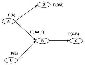
A Bayesian network is a graph model to estimate a complicated multivariate joint probability distribution through local probabilities [10,20]. Figure 1 shows a N = 5 nodes Bayesian network. The vertices represent genes or other components. They are random variables. The edges represent the conditional dependence relation and interactions among genes. For the set of parent nodes of a node , a conditional distribution is defined, where denotes the variables corresponding to the direct regulators of node.
In [18], the dynamic Bayesian network with external noise from time series is introduced. The influence of external noise on the systems dynamics is due to flipping of the value of a gene at each time step with a probability . The result shows that increasing the value of external noise can reduce the overall performance.
Linear additive regulation model with noise
In this model the expression level of a gene at a certain point can be calculated by the weighted sum of the expression levels of all genes in the network at a previous time point [11]. It may be represented by ODEs
Where is the gene expression level of the gene. N is the number of genes in the GRN. represents the effect of the gene on the gene. Negative means inhibition while positive represents activation. is the external (control) variable. represents the effect of the external variable on the gene. k is the number of external variable. is a bias term. In [21], the noise in the input data is considered in the linear additive regulation model. For each new input data, there is small amount of Gaussian noise with the same standard deviation added.
Neural networks model with noise
Neural networks model uses differential equations to describe GRN [13].
Where is usually a nonlinear function, such as a sigmoidal function. is the weight matrix. is the external (control) variable. represents the effect of the external variable on the gene. The constant represents the rate constant of degradation of the gene product . represents an external input. Neural networks can be used to assimilate the microarray data and construct GRNs [22]. In [23], Hierarchical Bayesian Neural Network model was introduced. Two kinds of noise are considered: independent parameters with Gaussian noise and correlated parameters with Multivariate Normal distribution. In [24], stochastic neural network models are presented for gene regulatory networks. The Poisson random noise is used to represent chance events in the process of synthesis. For expression data with normalized concentrations, exponential or normal random noise is used to generate the synthetic data.
Continuous Nonlinear Ordinary Differential Equations Model with Noise
A continuous nonlinear ordinary differential equation model is adopted. It includes random noise parameters from intrinsic noise and external noise which come from the noise source from gene regulating process. Compared to linear models, identification of the nonlinear ordinary equation model is computationally more intensive and can require more data; however, the range of nonlinear behaviors exhibited by GRNs can be more thoroughly understood with nonlinear differential equations. With more time-series data become available owing to advances in microarray or other biological technologies, and assuming continued improvement in computational capacity, it can be expected that continuous dynamic model will play a critical role in revealing complicated gene behavior.
Assuming there are N genes of interest and denotes the state (such as the microarray reading) of the gene, then the dynamics of the GRN may be modeled as
where is external noise.
In this study we assume the functions ( ) are in the form
where is the component of the nonlinear function , is the number of components in function. is parameter noise.
The proposed model includes all the major characteristics of a gene regulatory network: it is nonlinear, dynamic, and noisy. The rationale behind the proposed model are two-fold: first, the proposed model is general and sufficiently flexible to include many well-known models and new models yet to be found; second, the noisy nature of GRNs is modeled explicitly. The deterministic model (without noise) corresponds to the nominal case, while the various stochastic effects are included as noise disturbances. Previous work has modeled these noise types by Gaussian white noise processes [7]. The inclusion of noise also enables the proposed model to provide interpretation of the fact that GRNs are robust to noise, by which it is meant that the relationships among genes are not greatly affected by small changes caused by noise.
The nonlinear () need to be identified from time-series microarray measurements such that the identification error is minimized and the simplest model structure is selected. Both synthetic data and experimental data from microarray measurements are used to evaluate the proposed method. Note that although the proposed method is tested only using polynomials as the nonlinear terms, it is expected that it should perform similarly well for other choices of nonlinear terms in the proposed model, dependent of course on sufficient data for more complex nonlinear models.
The Algorithm for Noise Analysis in Polynomial Model, S-system model, and Microarray Data
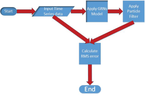
In this section, the polynomial model, S-system model, and particle filter are described in details. The algorithm for noise analysis inside gene regulatory networks is proposed on the basis of particle filter. The key steps of the proposed algorithm are shown in figure 2. The proposed algorithm is shown in details below.
Polynomial model
In this research, polynomials are chosen as the nonlinear components ( ) in the proposed model and ODEs with dynamic polynomials are used in our test cases. The polynomials are utilized as universal approximators. In order to mitigate the effect of "the curse of dimensionality", only second-degree polynomials are selected. Note that an advantage of using low-degree polynomial models is that even when there exists some model mismatch, these models may be sufficiently accurate to represent many real systems, and thus are widely utilized in practice [25]. We note that a similar GRN model has been adopted by [26], but without noise being included in the model. The polynomial model is given by:
where N is the number of genes, is the gene, , , and are constant factors.
S-system model
Inference of GRNs using S-system model from time-series microarray measurement data has attracted a lot of attention recently [27-30]. The S-system model is given by:
where is the index for the genes , are the state variables, and are the positive rate constants, and and are the exponential parameters called kinetic orders. If , gene will induce the expression of gene . On the contrary, gene will inhibit the expression of gene if . will have the opposite effects on controlling gene expressions compared to . The S-system is a quantitative model which is characterized by power-law functions. It has a rich structure capability of capturing various dynamics in many biochemical systems. In addition, the S-system model has been proven to be successful in modeling GRNs [30,28]. Hence, the S-system model is adopted for modeling GRNs in this study. Because the microarray data usually contain noise, it is very hard to pinpoint the exact values of the parameters. Hence, the determined parameters in the system were seen as some kind of distributions [30].
Particle filter
Particle filter is also called Sequential Monte Carlo (SMC) methods. Particle filter is a set of genetic-type particle Monte Carlo methodologies to solve the filtering problem [31]. It is a probability-based filter. The key idea is to generate a given number state vectors based on the probability density function (pdf) [31]. In particle filter, the microarray data is represented in terms of the variables , which are also a set of noisy observations. A state space model is given below.
The covariance of is , and the covariance of is .
The general procedure of particle filter is given by Algorithm 1.
Algorithm 1: The noise process of GRNs model on the basis of particle filter
Input: S-system function , the initial stage pdf (x0)
1: Generate M initial posteriori particles on the basis of the pdf (x0): M is the number of particles.
2: for do
3: Perform the time propagation step to obtain a priori particles
Where is generated on the basis of pdf of .
4: Compute the relative likelihood qj of each particle conditioned on the measurement of yi on the basis of non linear measurement equation (Polynomial and S-system models) and the pdf of the measurement noise
Where y* is a specific measurement, and L is the number of elements.
5: Scale the relative likelihoods
6: Resampling step: generate posteriori particles on the basis of the relative likelihoods qi
7: Compute the mean and covariance on the basis of
which are distributed according to the
pdf
8: end for
9: Estimate the RMS error
where is one specific measurement.
Noise analysis of microarray data using particle filter
The operations of proposed method to analyze noise in GRNs model using particle filter is graphically depicted in figure 2. The corresponding pseudocode of our method is summarized in Algorithm 2
Algorithm 2: The simulation procedure of GRNs model using particle filter
1: Generate data without any noise using Runge Kutta algorithm
Where h is the time step.
2: Generate data with system noise (Covariance is Q) and measurement noise (Covariance is R)
3: Apply particle filter on the noisy data to estimate the GRNs
4: Estimate the RMS error
Synthetic Simulation Results
The noise analysis method for GRNs models is tested by synthetic data using polynomial and S-system GRNs models.
Synthetic data simulation using polynomial model
In order to test the noise analysis procedure using particle filter, the synthetic network using polynomial model can be approximated as:
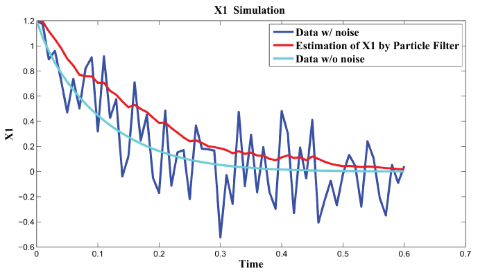
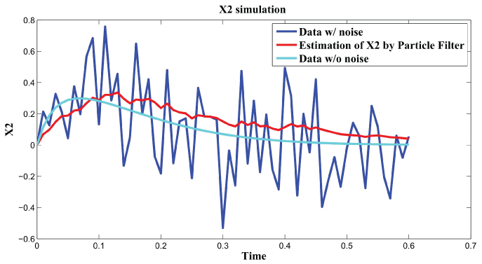
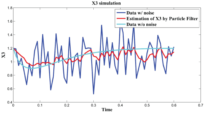
Figure 3, Figure 4, and Figure 5 show simulation results by particle filter. Genes , , and can be inferred under external and internal noise environment which make sure to find the relations among genes.
.
Figure 4: Synthetic simulation data for X2 with Noise Covariance Q = 10 and R = 0.08.
View Figure 4
In order to further analyze the noise relation to final results, RMS error is used to testify the effects of different noise level with and . The result is shown in figure 6. From the data and figure 6, we can see that RMS error is distributed within the interval when is in the range . RMS error is distributed within the interval when is in the range . We concluded that the effect of noise is larger than the effect of noise on the final results. In the research of [3], the observation that the time scale for intrinsic noise fluctuations is much shorter than that for extrinsic noise suggests that extrinsic noise may affect cellular phenotype more strongly than intrinsic noise at least in E. coli. Our results further confirmed this conclusion.
.
Figure 5: Synthetic simulation data for X3 with Noise Covariance Q = 10 and R = 0.08.
View Figure 5
Synthetic data simulation using S-system model
In order to examine the effectiveness of the proposed procedures for noise analysis in S-system using particle filter, a synthetic S-System model is used. The original S-system model is given as follows [30].
.
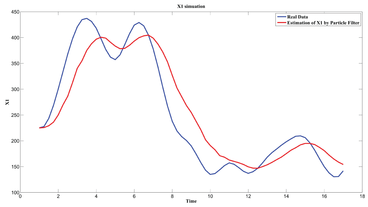
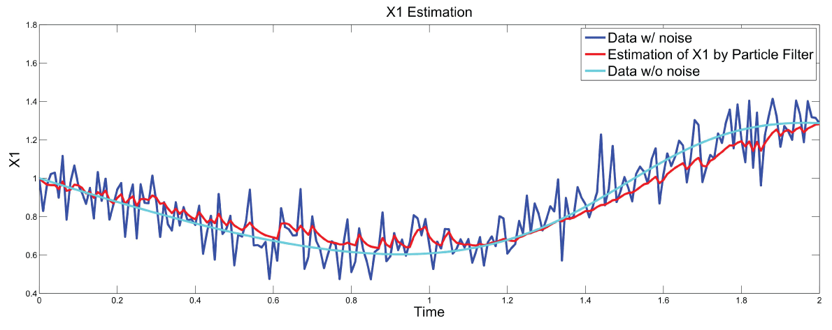
Figure 7: Synthetic simulation data for X1 with Noise Covariance Q = 10 and R = 0.1.
View Figure 7
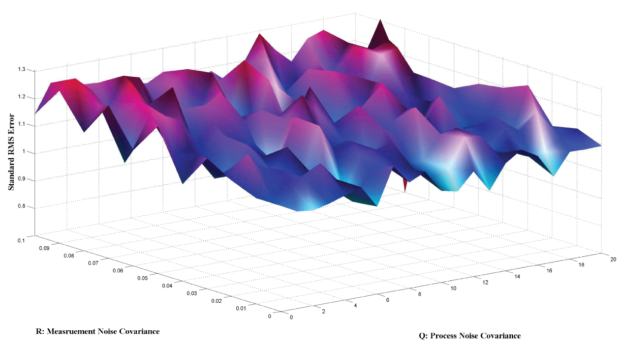
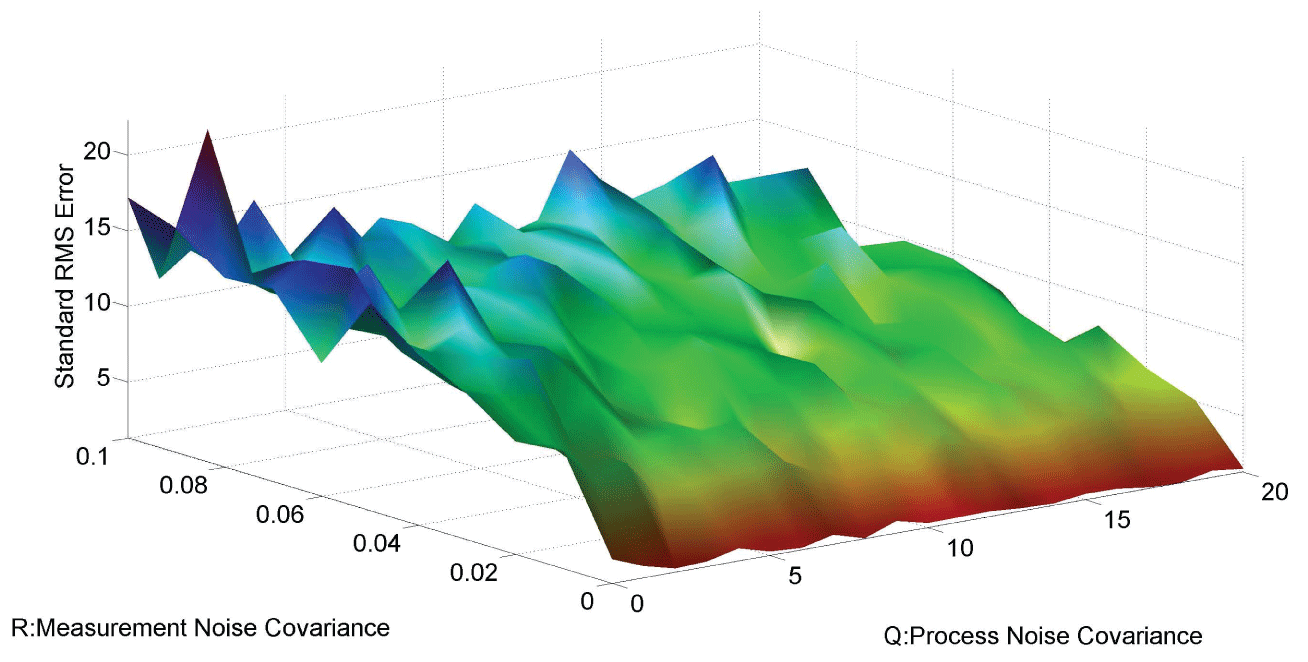
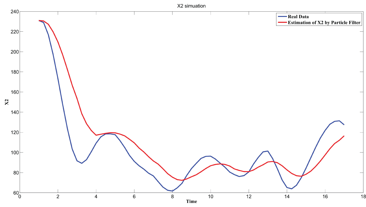
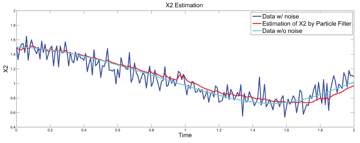
Figure 7 and figure 8 show simulation results using particle filter with noise levels by Q = 10 and R = 0.1. In the simulation, is equal to and the number of particles is equal to . We notice that particle filter can predict the system with an error so negligible that it cannot be realized by linear filters. Figure 9 shows the relations among RMS error, process noise covariance, and measurement noise covariance. When measurement noise covariance increases, the RMS error increases more. This indicates that the increase of measurement noise covariance can incur much more error than the process noise covariance.
.
Figure 8: Synthetic simulation data for X2 with Noise Covariance Q = 10 and R = 0.1
View Figure 8
Microarray Data Simulation
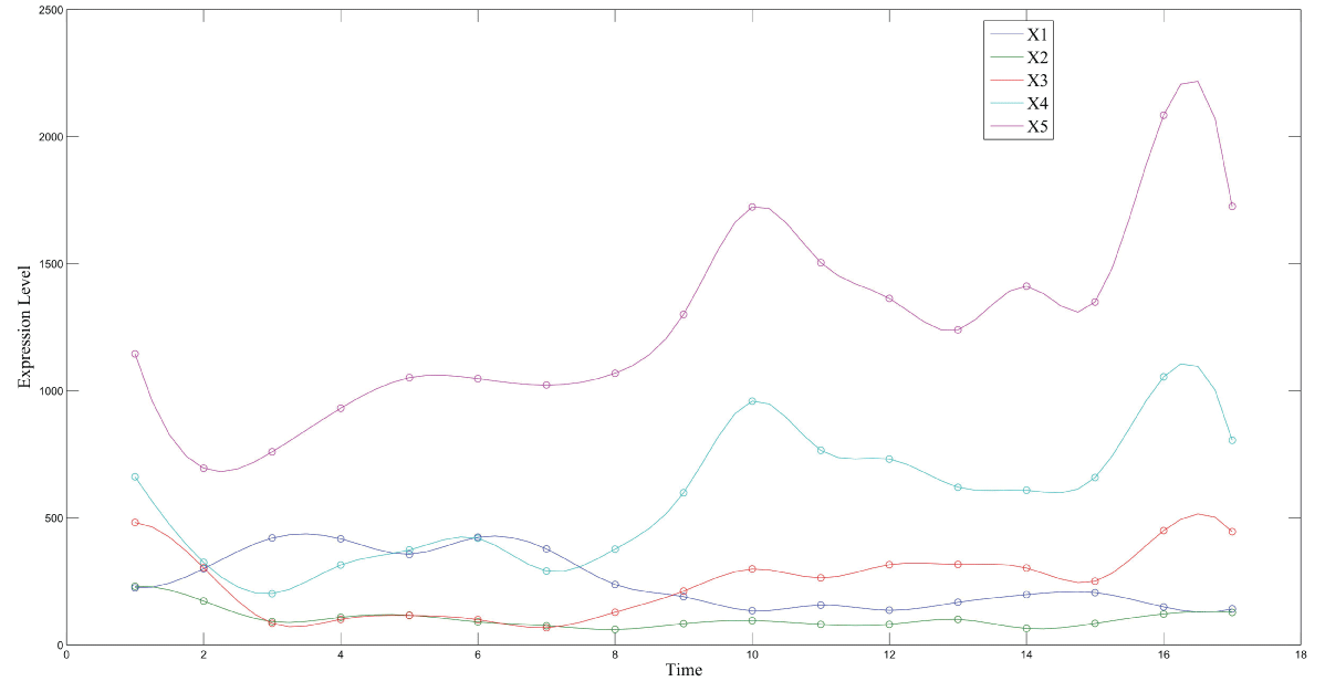
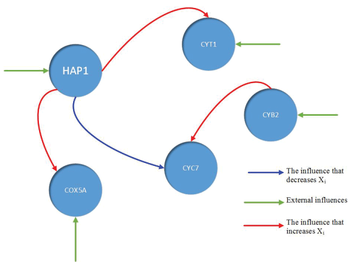
During this part of the simulation, time-series gene-expression data corresponding to yeast protein synthesis [32] are considered. Five genes (HAP1 (), CYB2 (), CYC7 (), CYT1 (), COX5A ()) are selected because the relations among them have been revealed by biological experiments. The relations are shown in figure 10 with noise.
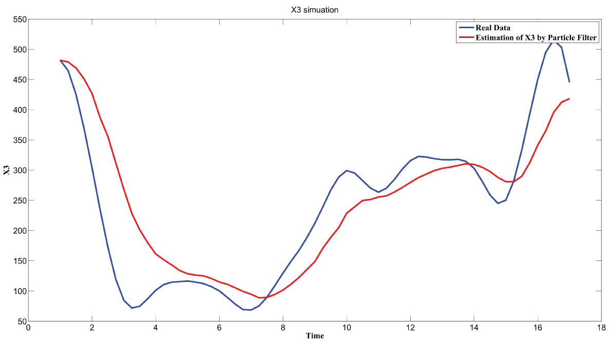
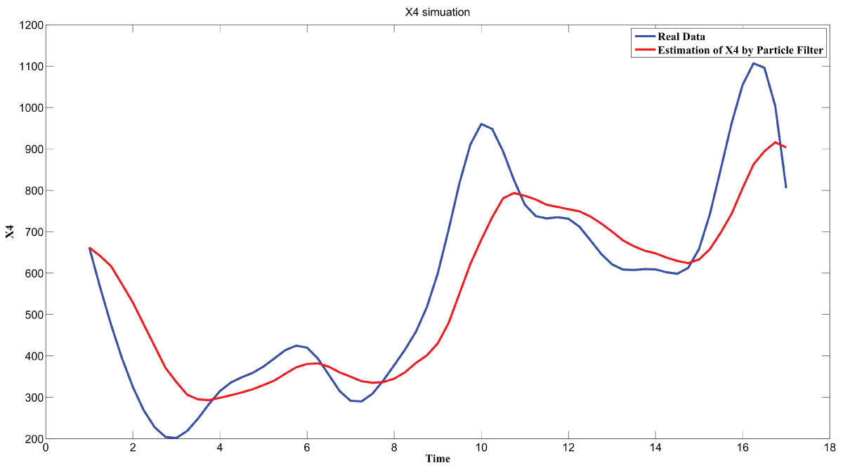
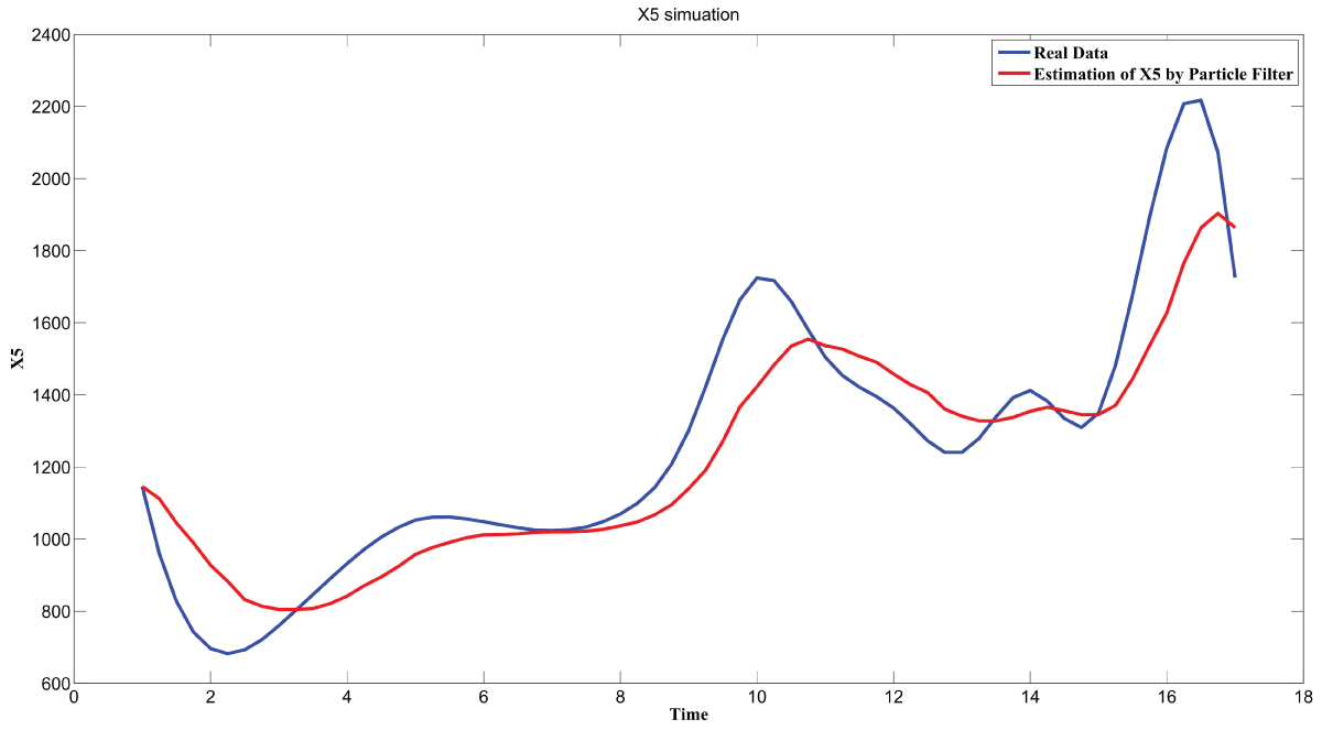
Particle filter is applied to analyze the data with noise. The particle filter estimate is the mean of particles which caused the time shift or delay on the curve. It is inherent in particle filter and is called mean shift.
The result is shown by figure 11, figure 12, figure 13, figure 14, and figure 15 for genes HAP1, CYB2, CYC7, CYT1 and COX5A. The branch pathway model is shown by figure 16 on the basis of the above results.
The relations are in agreement with the biological experiment findings in [33].
Conclusions
In this paper, process noise and measurement noise of gene regulatory networks is analyzed using particle filter. The synthetic models on the basis of polynomial and S-system are studied to analyze the relations among RMS, measurement noise, and process noise. We found out that measurement noise is the main reason to incur the RMS error conforming to results from biological experimental research. Noise inside microarray data is considered and analyzed with five real genes.
Acknowledgement
The work of Haixin Wang and Dawit Aberra was supported by NSF Grant 1435152.
References
-
Swain PS, Elowitz MB, Siggia ED (2002) Intrinsic and extrinsic contributions to stochasticity in gene expression. Proc Natl Acad Sci USA 99: 12795-12800.
-
Tao Y (2004) Intrinsic and external noise in an auto-regulatory genetic network. J Theor Biol 229: 147-156.
-
Raser JM, O'Shea EK (2005) Noise in gene expression: origins, consequences, and control. Science 309: 2010-2013.
-
Hooshangi S, Weiss R (2006) The effect of negative feedback on noise propagation in transcriptional gene networks. Chaos 16: 026108.
-
Lei J (2009) Stochasticity in single gene expression with both intrinsic noise and fluctuation in kinetic parameters. J Theor Biol 256: 485-492.
-
Kaern M, Elston TC, Blake WJ, Collins JJ (2005) Stochasticity in gene expression: from theories to phenotypes. Nat Rev Genet 6: 451-464.
-
Hasty J, Pradines J, Dolnik M, Collins JJ (2000) Noise-based switches and amplifiers for gene expression. Proc Natl Acad Sci USA 97: 2075-2080.
-
Tao Y (2004) Intrinsic noise, gene regulation and steady-state statistics in a two-gene network. J Theor Biol 231: 563-568.
-
R Pal, A Datta, E R Dougherty (2006) Optimal Infinite Horizon Control for Probabilistic Boolean Networks. Signal Processing, IEEE Trans 54: 2375-2387.
-
Zou M, Conzen SD (2005) A new dynamic Bayesian network (DBN) approach for identifying gene regulatory networks from time course microarray data. Bioinformatics 21: 71-79.
-
D'haeseleer P, Liang S, Somogyi R (2000) Genetic network inference: from co-expression clustering to reverse engineering. Bioinformatics 16: 707-726.
-
H Ressom, D Wang, R S Varghese, R Reynolds (2003) Fuzzy Logic-Based Gene Regulatory Network. The IEEE International Conference on Fuzzy Systems.1210-1215.
-
E keedwell, A Narayanan, D Savic (2002) Modeling Gene Regulatory Data Using Artificial Neural Networks. Proceeding of IEEE 1: 183-188.
-
H Lahdesmaki, I Shmulevich, O Yli-Haerja (2004) On Learning Gene Regulatory Networks under the Boolean Network Model. Machine Learning 52: 147-167.
-
Shmulevich I, Dougherty ER, Zhang W (2002) Gene perturbation and intervention in probabilistic Boolean networks. Bioinformatics 18: 1319-1331.
-
X Zhou, X Wang, E Dougherty (2003) Construction of genomic networks using mutual-information clustering and reversible-jump Markov-Chain-Monte-Carlo predictor design. Genomic Signal rocessing 83: 745-761.
-
Kim H, Lee JK, Park T (2007) Boolean networks using the chi-square test for inferring large-scale gene regulatory networks. BMC Bioinformatics 8: 37.
-
F E Streib, M Dehmer, Bakir GH, Muhlhauser M (2005) Influence of Noise on the Inference of Dynamic Bayesian Networks from Short Time Series. ENFORMATIKA 10: 70-74.
-
Akutsu T, Miyano S, Kuhara S (2000) Inferring qualitative relations in genetic networks and metabolic pathways. Bioinformatics 16: 727-734.
-
T Chen, V Filkov, S S Skiena (2001) Identifying gene regulatory networks from experimental data. Parallel Computing, Elsevier Science Publishers, The Netherlands 27: 141-162.
-
P D'haeseleer, S Fuhrman (1999) Gene Network Inference Using a Linear, Additive Regulation Model.
-
R Xu, D Wunsch (2005) Gene regulatory networks inference with recurrent neural network models. IEEE International Joint Conference 1: 286-291.
-
Liang Y, Kelemen AG (2004) Hierarchical Bayesian neural network for gene expression temporal patterns. Stat Appl Genet Mol Biol 3: Article20.
-
T Tian, K Burrage (2003) Stochastic Neural Network Models for Gene Regulatory Networks. IEEE Evolutionary Computation 1: 162-169.
-
Nelles (2001) Nonlinear System Identification. Springer.
-
S Ando, E Sakamoto, H Iba (2002) Evolutionary Modeling and Inference of Gene Network. Information Science 145: 237-259.
-
Kepler TB, Elston TC (2001) Stochasticity in transcriptional regulation: origins, consequences, and mathematical representations. Biophys J 81: 3116-3136.
-
S Kimura, M Hatakeyama, Akihiko Konagaya (2004) Inference of S-system models of genetic networks from noisy time-series data. Chem-Bio Informatics Journal 4: 1-14.
-
Kutalik Z, Tucker W, Moulton V (2007) S-system parameter estimation for noisy metabolic profiles using newton-flow analysis. IET Syst Biol 1: 174-180.
-
Wang H, Qian L, Dougherty E (2010) Inference of gene regulatory networks using S-system: a unified approach. IET Syst Biol 4: 145-156.
-
D Simon (2006) Optimal State Estimation Kalman, H_inf and Nonlinear Approaches. John Wiley & Sons.
-
H Wang, L Qian, E Dougherty (2007) Inference of Gene Regulatory Networks using S-System: A Unified Approach. IEEE 2007 Symposium on Computational Intelligence in Bioinformatics and Computational Biology.
-
Schneider JC, Guarente L (1991) Regulation of the yeast CYT1 gene encoding cytochrome c1 by HAP1 and HAP2/3/4. Mol Cell Biol 11: 4934-4942.


