International Journal of Clinical Biostatistics and Biometrics
A Review of Graphical Approaches to Common Statistical Analyses. The Omnipresence of Latent Variables in Statistics
Emil N. Coman1*, L. Suzanne Suggs2, Maria A. Coman4, Eugen Iordache3 and Judith Fifield1
1TRIPP/HDI, University of Connecticut Health Center, USA
2University of Lugano, Switzerland
3Transilvania University, Romania
4University of Connecticut, USA
*Corresponding author:
Emil N Coman, University of Connecticut Health Center, Farmington, Connecticut, USA, E-mail: coman@uchc.edu
Int J Clin Biostat Biom, IJCBB-1-003, (Volume 1, Issue 1), Review Article; ISSN: 2469-5831
Received: July 31, 2015 | Accepted: September 02, 2015 | Published: September 04, 2015
Citation: Coman EN, Suggs LS, Coman MA, Iordache E, Fifield J (2015) A Review of Graphical Approaches to Common Statistical Analyses.The Omnipresence of Latent Variables in Statistics. Int J Clin Biostat Biom 1:003. 10.23937/2469-5831/1510003
Copyright: © 2015 Coman EN, et al. This is an open-access article distributed under the terms of the Creative Commons Attribution License, which permits unrestricted use, distribution, and reproduction in any medium, provided the original author and source are credited.
Abstract
We provide a comprehensive review of simple and advanced statistical analyses using an intuitive visual approach explicitly modeling Latent Variables (LV). This method can better illuminate what is assumed in each analytical method and what is actually estimated, by translating the causal relationships embedded in the graphical models in equation form. We recommend the graphical display rooted in the century old path analysis, that details all parameters of each statistical model, and suggest labeling that clarifies what is given vs. what is estimated. We link in the process classical and modern analyses under the encompassing broader umbrella of Generalized Latent Variable Modeling, and demonstrate that LVs are omnipresent in all statistical approaches, yet until directly 'seeing' them in visual graphical displays, they are unnecessarily overlooked. The advantages of directly modeling LVs are shown with examples of analyses from the Active8 intervention designed to increase physical activity.
Introduction
Research in a variety of fields including medicine and social sciences makes use of statistical tests that have a long tradition and have become almost second nature to researchers and methodologists. Newer approaches to investigating truly causal connections between variables meant to explain and predict the causal nature of relationships are still developing however [1], but in the past decades one overarching statistical model rooted in causal modeling has expanded to include practically any imaginable statistical analysis. This approach is called the Generalized Latent Variable Model (GLMM [2-4]) and is a form of linear parametric statistical modeling that encompasses most known analyses, but does so while making latent variables (LVs) explicit and modeling them in the open.
We provide examples of classic and more modern analyses customarily used in answering broad research and statistical questions, and do so by detailing a visual method of depicting the statistical assumptions and expectations behind GLMM models, so that readers with varied backgrounds can translate them easily in their field, both when designing studies and when analyzing data and interpreting them. The visual method of describing linear (and nonlinear) causal relationships between true concepts and measured variables was invented by Sewall Wright almost a century ago [5] and offers more than just a graphical means of translating testable equation into visual models, it provides the framework for a comprehensive statistical approach that has rather few known limits [6]; it is also known as structural equation modeling (SEM) [7,8].
Analyses and their Visual Representations
The GLMM method centers on modeling latent variables, or LVs, and connects observed variables and LVs in causal (structural) models that promise a stronger causal inference footing compared to other statistical approaches [9-11]. GLMM is a parametric case of the more general nonparametric graphical causal language [12], which has evolved into a full-fledged causal calculus [13], known as structural causal modeling (SCM [14]). We restrict our review to the parametric structural models with continuous variables for simplicity, but we cover categorical LVs in the process; software and statistical advances however accommodate easily other types of outcomes (e.g. binary and counts [15]).
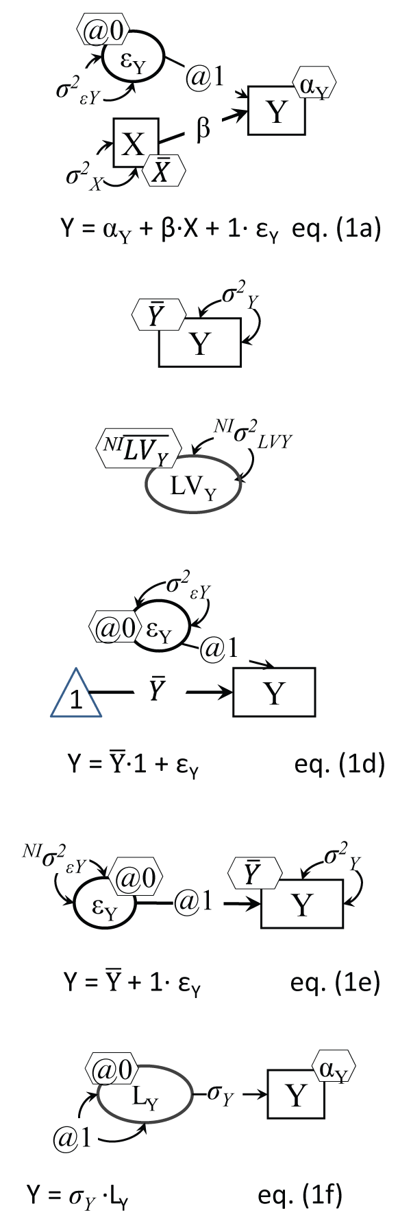
A latent variable is simpler to conceive of and view than one may think: it is just a variable that happened to be unobserved in one instance [16]; in this sense it is just a variable that is completely missing, whose values are not in the dataset. Figure 1b and Figure 1c depict the similarity between an observed Y and a latent Y (both continuous normally distributed): they are both described by their own mean and variance, it just happens that the raw data does not have any values for the LV in it. If one wants to 'see' such an LV, they can do so by simply generating a normally distributed score, easily done in Excel for example; by typing something like "=NORMINV(RAND(),0,1)", you just observed a score for one case of a latent variable with mean zero and variance one (these values can be changed at will); by typing it in say 100 cells in the same column, you have just 'observed' 100 cases (a sample), and when pressing 'Enter', all these 100 values are 'updated", i.e. a new sample with a new set of 100 values is 'drawn' for you from a population of infinite size.
.
Figure 1a : Simple regression as a structural model
Notes: Five parameters are estimated: αY (Y intercept): and
(X mean), σ2εY and σ2X , and of course the focal β, from five 'input' data points: the means and variances of X and Y, and their covariance; hence df = 0 for this model (i.e. it is saturated).
Figure 1b: An observed normal variable
Note: The mean
is attached to the Y variable rectangle in a hexagon.
Figure 1c: A latent normal variable
Note: The mean
and variance σ2 are not identified from this model, i.e. need to be specified/set, or the model needs to be expanded to estimate them, like in Figure 2b or Figure 6b.
Figure 1d: An observed normal variable 'regressed' on a constant of 1's
Note: The triangle is a 'variable' made up of 1's (a constant technically).
Figure 1e: An observed normal variable with error only as 'predictor'
Note: Variability in Y around its mean
is due solely to random error εY; NI indicates this parameter is non-identified, i.e. cannot be estimated in this setup.
Figure 1f: Variable Y model estimating its standard deviation (SD)
Note: Two parameters are estimated here: αY and σY (instead of the regular variance σ2Y).
View Figure 1
The direct analogue of this operation in software like Amos 5 ([17] or later) for instance is simply drawing a circle. That's all! Plus, of course, telling the program the same thing, which is that you know its mean (zero) and its variance (one), because no program could estimate them without any individual case values. Similarly, in Mplus for instance, one just writes a one line code like "LV by;", which is a short version of defining a latent variable by its indicators (like "LV by X Y Z;"), only in this case there are no such indicators of it; same as above, you need to tell the program that you know its mean and its variance (LV@1; [LV@0]), This happens to be in fact the shortest possible introduction to generating unobserved variables, or designing studies using Monte Carlo simulations: one creates variables with desired distributions from scratch and then can analyze them subsequently [18]; of course when connecting such a new LV to other variables (observed or not) one also needs to define the scale for all LVs, i.e. the unit of measurement (lbs., or inches, or a 1-5 disagree-agree scale, etc.). We present next several common and modern analyses using the graphical intuitive method that brings LVs to light.
On rules to translate structural models
First, we note that we visually specify in this paper the models with enough detail to stand on their own, with no equation necessary: equations can be fully derived from the visual models by following simple intuitive rules; we derived them for readers to ease the process. The models represent variables as network vertices (dots, or boxes) and the coefficients linking variables as lines with arrowheads, a method almost a century old [5,19]; we note that the arrows do more than just point, they convey 'causal directionality' [14]. Single headed arrows indicate a causal effect, while double headed arrows between variables stand for some common cause, omitted in the current model.
Because a normally distributed random variable (the focus of this review of methods) is fully described by its mean and variance, we represent variances as double headed arrows with arrows pointing to themselves, and the mean (or when the variable is caused by others, the intercept) by a small hexagon attached to the variable (see Figure 1b); while this may appear to complicate the display, compared to other current options (like Figure 1d, common in J. J. McArdle's research e.g. [20]) it will prove to really simplify things when models increase in complexity. Instead of the triangle of 1's, we choose to add a hexagon to each variable, for its mean (or intercept); εY stands for more than just error, it is commonly called a disturbance, and it encodes in fact all other factors affecting Y, not shown in this model. In fact, the double headed arrow pointing to the same exogenous (primary predictor) variable carries the same meaning of variability (or co-variability with itself) unexplained by the model, left to be explained possibly by larger causal models.
We distinguish between estimated and fixed model parameters, so that only one such visual depiction would be needed to represent both the input and the output (estimates) of a statistical model. When a residual error is specified for instance, like in Figure 1a, which translates visually a simple regression of Y on X, its loading is set to 1, labeled '@1' (to define its scale identical to its observed 'anchor' Y), and its mean is set to zero (because it cannot be identified otherwise); the direct equation translation of a structural model is then obtained by simply selecting an effect (Y) and adding up its causes (predictors), multiplied by their respective path/causal coefficients, e.g. for Figure 1a Y= αY + β.X + 1.εY. Note that the equation form has less information than the visual model, because one has to also acknowledge in equation form the assumptions Y = 0 and ρXεY = 0. We remind the reader that in a regression the variance of the predicted variable is not a model parameter, instead the variance of its residual error is estimated; similarly its actual mean is not estimated, but its intercept is, i.e. its mean if/when the predictors become zero.
Simple Variability Depictions
Continuous normally distributed variables can be directly represented as in Figure 1b or Figure 1c, described by two parameters: mean and variance; while these can be estimated from their sample counterparts for the observed Y, they cannot be derived for the latent LVY, i.e. they are not identified. So for LVs they will need to be either set to specific values, or will need some anchors to be derived from them, like using one or more indicators.
The Figure 1a regression model can be better grasped by stepping back and looking at even simpler models, like a single variable one. Figure 1b and Figure 1c display an observed Y and a LV latent counterpart, while Figure 1d depicts an alternative one variable model with the variable Y mean shown as a coefficient of the regression of Y on an (imaginary) constant variable with 1's for every case, hence formally: Y = .1 + 1.εY. The direct equation translation of Figure 1e is also simply Y = + 1.εY, with the corollaries E(Y) = E(εY), and σ2Y= σ2ε. Some common SEM software (like Mplus [15]) point out in their output which parameters were not estimated because were fixed to a certain value, by the user or by default: they have a standard error of zero, and hence a p value of practically one.
There is also a way to directly estimate in an LV model the standard deviation of a variable, like Figure 1f (as suggested in [21] or [22].
Measurement Error
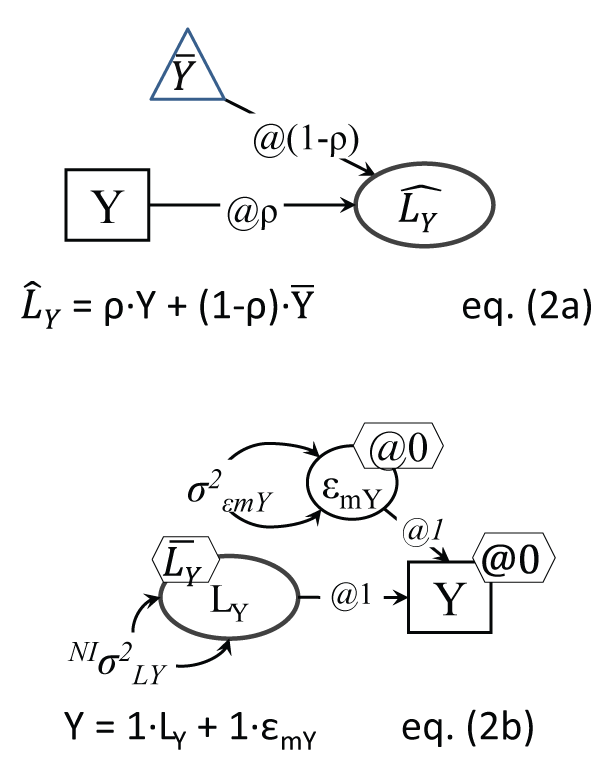
Estimating causal relationships between observed variables instead of using the true (latent) ones biases the true relationships, e.g. a 20% measurement error in a predictor variable X reduces by that much the estimate of the impact of X on an outcome Y [23]. A classic 'model' (not testable in the SEM sense) of the true scores is Kelley's equation, represented in Figure 2a [24] (cited in [25]), but a more direct testable model is in Figure 2b, which implies that the observed variable has a measurement error variance part σ2εmY (noise) that makes it not fully reliable (reliability is always ρ < 1). The equation in Figure 2b resembles a 'mini factor analysis' with only one indicator Y of the latent factor LY. Note that if the true LY is categorical (like ill vs. not ill), and Y is also categorical, the measurement error takes the form of a misclassification ([4]; such a model is presented later in Figure 9a).
.
Figure 2a: Kelley true score 'model'
Note: This setup is not a testable model, it depicts the contribution of the mean (as a constant, i.e. same values, in a triangle) and observed score into the true Y score, knowing the variable's reliability ρ.
Figure 2b: Variable Y with measurement error
Note: The residual error εmY is measurement error; one of course cannot identify from just two sample estimates (σ2Y and
) both: 1. σ2εmY and σ2LY; and 2.
and
. One of each needs to be fixed; commonly Y intercept is made 0; NI indicates this parameter is non-identified, i.e. cannot be estimated in this setup; the unreliability σ2εmY can be set to a reasonable share of the sample variance σ2Y, like 10-20% of it.
View Figure 2
The reader can notice that the one-variable (no measurement error) model in Figure 1b can be derived from the Figure 2b model by simply 'erasing' its measurement error variance, by setting the variance of σ2εmY to zero (its mean is assumed zero by default, because it cannot be identified). More generally in fact, it has been noted that LV models can be viewed as a sensitivity analysis of their simpler observed variable-only counterparts ([4]).
Now that we can see how models can be translated into equations and statistical tests, we can pursue the example of specific statistical analyses. We will briefly describe each, and depict their visual display, but we mention first briefly the study that provided data for these illustration. Active8 was a randomized controlled trial (RCT) with two intervention groups in which identical physical activity-promoting messages were delivered using either email or SMS; more details are in [26]. In these analytic examples we used two variables measured at baseline and after 12 weeks, moderate physical activity (PA), in days per week, and attitudes towards PA. All our analyses with output details and a fully deidentified extract of the data used in these examples are posted as online appendix at http://trippcenter.uchc.edu/modeling and http://bit.ly/1DKSmB1
t-test and Anova
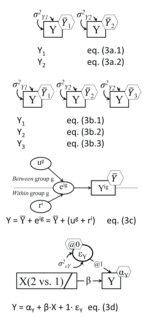
Comparisons between means of a continuous outcome can be achieved with a direct test of significance of the difference between means, as with the t-test, or by comparing the between-group to the within-group variability, as in Anova. The two analyses will yield identical results in terms of significance of the difference in means for two-group comparisons. We tested the difference in means of the last wave outcome measure, moderate physical activity (PA) at work, in the entire sample (both conditions), with a t-test and an F test (Anova), which are related of course like t2 = F, and should coincide in terms of significance; they did in fact: p = .547, with t(80) = - 0.605 and F(1,80) = 0.37. A more direct view of these tests is shown in Figure 3a and Figure 3b; these are in fact easily testable models in software like AMOS or Mplus: they are 1-variable two (or more) group models, and hence with as many parameters as groups to be compared, and they can test equalities of parameter hypotheses by imposing equality constraints and testing whether the model drops in fit dramatically (case in which we reject the equality just imposed). Note that since there are variances estimated in each group, and the 'baseline' model, against which we test the equality of means hypothesis, needs to be a well-fitting model, one may have to allow at times the group variances to be equal, or not [27].
.
Figure 3a: The t-test model
Note: The independent samples t-test is testing the hypothesis:
=
; this two-group setup allows for inclusion of group specific covariates; the two equations are simply one variable for each group, but across-group constraints are possible, like σ2Y1 = σ2Y2.
Figure 3b: Anova depiction as multiple-group model
Note: Anova results are identical to testing in a multiple-group model and
=
=
= ...etc.; the multiple-group setup allows for inclusion of group specific covariates; there is only one Y variable, with 3 means and variances.
Figure 3c: The Anova error decomposition
Note: Variable Y varies across both groups (indexed by g) and individuals (indexed by i); one case's score then deviates from its own group mean, such deviations contributing to the variance of ri, and group means differ from the grand (overall) mean, which is captured by the variance of ug.
Figure 3d: The Anova model as regression
Note: Being in group 2 (vs. 1) leads to having different Y outcome means; β reflects the difference in Y means; the bar in the X rectangle indicates a categorical variable; with more than 2 groups, several contrast dummy coded groupings can predict Y.
View Figure 3
We detail in the online appendix the AMOS t-test equivalent as a 2-group one variable model, which clearly demonstrates the flexibility of this approach, by testing the 'equality of means' hypothesis against different baseline models: assuming variances to be equal, or different; the results are replicated in the sub-sample with valid Y values. Another level of flexibility involves combining the Figure 2b and Figure 3a models; this means that one can test for equality of means in a two-group AMOS model by relying on the true variances (and hence standard deviations), because true variances are only a part (albeit the largest) of an observed variable's variance, with the rest being noise, or measurement error [28]. Such a test allows one to assess the sensitivity of the t-test to a range of plausible reliability values in each group; assuming a small unreliability of 10% in both groups e.g. did not alter the p value in our case.
Another way to intuitively grasp the logic of Anova is to depict the decomposition of the error of a variable into its between-group and within-group components, as in Figure 3c. In fact this decomposition is the basis of two-(and multiple) level models, which in Mplus for example are run with no other model specification than 'Analysis: Type=basic twolevel;'. Anova can of course be tested using a regression setup [29], using binary predictors to contrast the groups that are the focus of comparison (see Figure 3d); this setup confesses openly the causal assumptions behind the analysis, i.e. that the grouping variable is the source (cause) of the differences in means of the 'dependent variable', as it is specifically labeled in software like SPSS [30].
The Paired t-test and Repeated Measures Anova (RAnova)
Testing whether a significant change occurred is often done with a paired t-test, which has been shown however to be fully replicated (as a particular case) by an LV model that has the change between time points directly specified as LV in the model [31] (we detail it below in Figure 5a). A paired t-test for the baseline-> 12 weeks moderate PA changes for example indicated a significant increase overall in the whole sample (N = 49, for valid pairs of observations baseline and follow-up), t(48) = -2.252, p = .029, for an average increase of .469, from a 2.673 average to a 3.143 average of days of moderate PA at work. A RAnova test of the same changes yielded a F(1,48) = 5.07, with the same p value of course.
.
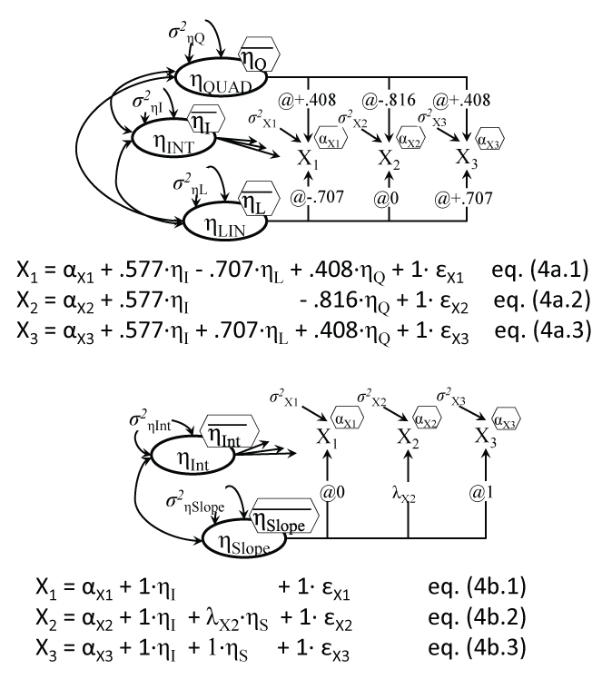
Figure 4a: Repeated ANOVA as latent growth model
Note: All three coefficients from intercept factor η are set to .577.
Figure 4b: Latent growth model with linear and quadratic trends
Note: The three coefficients from intercept factor η are set to 1; the middle loading is estimated, instead of fixed, to model curvilinear trajectories of any shape; the linear slope is centered on time 2.
View Figure 4
.
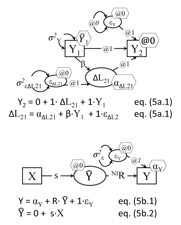
Figure 5a: Latent Change Score model (replicating paired t-test and 2-wave Ranova)
Note: Many parameters are fixed here (see @ signs), leaving to be estimated only the intercept and residual variance of the LCS score ΔL21, the mean and variance of the baseline Y, and the proportional growth parameter β.
Figure 5b: Regression with the predicted outcome
in the model
Note: s is a structural coefficient; the β regression coefficient for the Y on X regression is β = s.R; one cannot estimate both R and σ2ε, but they are related because R2 is the explained Y variance (when R is standardized) and σ2ε is the unexplained Y variance, so they sum up to 1.
View Figure 5
Latent Growth Models
It has been shown before that models of change are overlapping, and that growth models with specific constraints replicate both the paired t-test and repeated measures Anova (RAnova) models [32]. A LGM replication of a RAnova test is has been detailed by Duncan [33] and Voelkle [32], and it involves fixing the loadings linking the slope factor, i.e. the individual score capturing the average change for each individual in the sample, to the observed scores, to values representing the polynomial coefficients used in RAnova. We show them for 3 waves of data in Figure 4a, an illustration of a LGM with both linear and quadratic growth (latent) factors.
LGMs can have more flexibility than RAnova, by allowing for instance free-shape trajectories of change, like Figure 4b, by freeing the middle loadings λ. For the moderate 3 wave physical activity (PA), the model indicated a significant average increase (slope) of .603 days/week (SE = .227), p = .008. The estimated middle loading turned out to be .806 (.350), p = .021, which for our equal time interval means that by 6 weeks (the middle time point) 81% of the final change was already achieved. Note that although the model does not make this explicit, LGM is in fact a 2-level (hierarchical) model, with level 1 measures and relations (X1-X3 and their regressions on ηINT and ηLIN and ηQUAD), while the regressions of η's on their own predictors (if any are specified) are technically level-2 relations [34].
The visual SEM models make clear what assumptions are relied upon in analyses like RAnova. They especially clarify the expectations about the relationships between residual errors made e.g. in mixed linear models (examples from Stata and SPSS are in the online appendix). These assumptions may range from an unstructured pattern (error variances and covariances between them all free) to compound symmetry (variances equal, and covariances between any pair of errors equal), to autoregressive patterns (variances equal, covariances decreasing for further away pairs); such constraints are handled easily in SEM software.
LGM in its structural form makes these 'input' settings more visible, besides it can also formally test such assumptions, and adds the possibility of adjusting the model based on how much the model specifications depart from data (beyond checking the model fit); for example often LGM will lead to negative variances of some observed repeated measures residuals, which can be by-passed by setting those variances to zero (and then accepting a non-positive definite matrix' warning, i.e. covariances between the offending error and other variables cannot be defined).
Latent Change Score models
We have shown before that the latent change score (LCS) can fully replicate the paired t-test [31], and since latent growth models (LGM) are a particular case of LCS ones [35], LCS can handle LGMs and then can even expand them with additional features (like dynamic relations). While the LCS setup in Figure 5a may appear complex, the model is rather intuitive: a change score (as an LV however, not a mere calculated difference score) is created by tricking the software into literally doing the desired subtraction ΔL21 = Y2 - Y1, but by adding up two causes of the later variable Y2: the prior values Y1 and the 'change mechanism' ΔL21: Y2 = ΔL21 + Y1.
Many parameters are set to 0 or 1 to setup this subtraction, but LCS models have a host of advantages, among them modeling complex trajectories of changes and accounting for how changes depend on their prior values, as well as on other variables' prior values and even on prior changes [36,37]. LCS models can also uncover complex dynamic processes induced by interventions or treatments [38]. The LCS model run in Mplus replicated the paired t-test and Ranova results, when the LCS model was restricted to a subsample of cases with values valid for both waves however; the intercept of ΔL21 (i.e. the average change at zero predictor values, which of course was centered) was .470 (SE = .189), p = .013.
When the entire sample was analyzed however, the operant sample size for the baseline->12weeks LCS model of change increased (to N = 194), because software like AMOS and Mplus use what is known as Full Information Maximum Likelihood (FIML), which in essence uses information even from cases with only baseline or only follow-up valid values in estimating the model parameters, which is a proven advantage of FIML estimation [39]. FIML yielded the ΔL21 intercept as αΔL21 = .414 (SE = .160), p = .009; we confirm the conclusion that this outcome increased significantly.
Before moving into presenting several more complex statistical models, we briefly mention another way of seeing an underlying (unobserved) variable that is referred to in regression analyses, which is the key element in all models we showcase; it was suggested by Graham [40]. He presented the model that we adapted in Figure 5b, which illustrates the distinction between the actual observed Y and the predicted outcome; this model is not identified (not all parameters can be estimated without additional constraints imposed). We note again that visual LV models can better clarify the inner workings of such statistical analyses.
The Factor Model
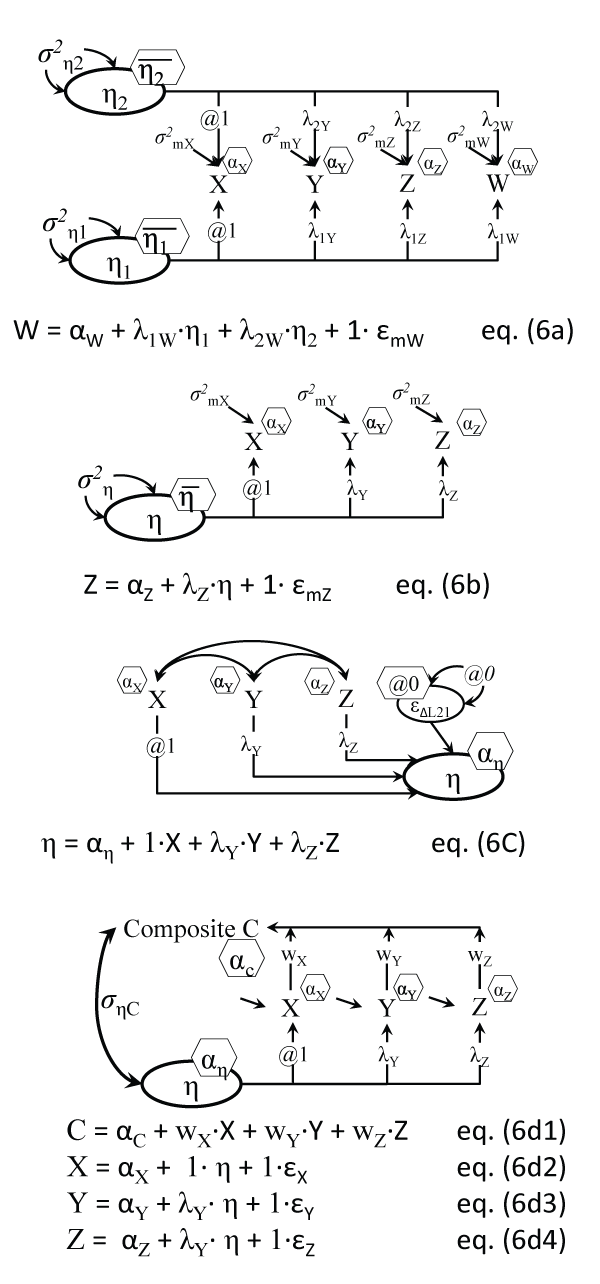
A commonly used statistical analysis directly makes reference to LVs and specifies them. Factor analysis investigates in its exploratory and confirmatory modes latent structures of the observed variables, by uncovering unobserved variables or LVs, called common factors. The LV factors account for the common variability (covariances) between observed variables [7]. The EFA and CFA models are illustrated in Figure 6a and Figure 6b. An EFA of the 6 'attitude about physical activity' (PA) items (same three items, three from baseline and three from follow-up) successfully separated out the two sets by time, i.e. the two factors extracted were mapped unto their respective waves (see online appendix for details). A CFA of the three baseline attitude towards PA items yielded standardized loadings of .74, .80, and .69; note that the first loading in Figure 6b is set equal to one, in its unstandardized form.
.
Figure 6a: Exploratory Factor Model (2 factors shown)
Notes: Indicators are uncorrelated, given/(conditional on) their common predictors η1 and η2. In EFA the number of factors is not known a priori; η1 and η2 can be correlated or not; only the equation for the last indicator is shown; ε ellipses are replaced by residual variances σ2.
Figure 6b: Confirmatory Factor Model (scale)
Note: Indicators are uncorrelated, given/(conditional on) their common predictor η; only the equation for the last indicator is shown.
Figure 6c: Causal indicators model (index)
Note: The residual error variance of the formative factor is commonly set to zero.
Figure 6d: Factor model with composite (computed, i.e. observed) score
Notes: Errors and intercepts are omitted for clarity; C is neither a full square nor an oval, as it's a score computed from observed indicators; ((σηC)2 is the reliability of C, i.e. proportion variance of C explained by η.
View Figure 6
We remind readers that there exist also formative measures, i.e. causal indicator measures, shown in Figure 6c, for concepts like SES, who are literally composed of their ingredients, rather than looming behind them as their underlying cause [41]. Also, it is possible to test the reliability of computed composite scores (like weighted or unit weight total scores) by directly linking the two variables, the LV factor score and the composite that now is (partially) observed, like in Figure 6d; this was suggested by [42], but see [43] for an example.
LCA Latent Class Analysis
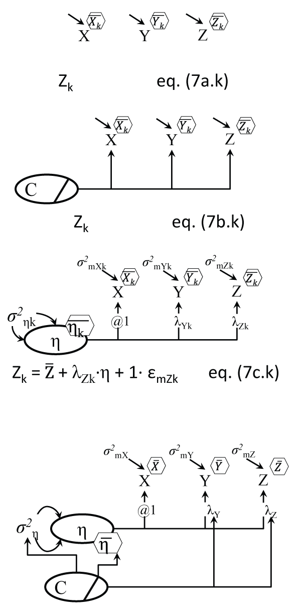
Latent Class Analyses attempt to explain the observed covariances between variables through the existence of distinct classes of cases (participants) within which such covariances disappear. A 2-class LCA analysis for example of the three baseline attitude items extracted classes of 84 and 205 cases, differing in terms of all three of their item averages of course, which were all lower in the first class and higher in the second, respectively. Expectations about the equality (or not) of variances of each indicator variable (X, Y and Z) can be specified; note that the Figure 7a model differs from the Anova Figure 3b model only by the LCA model having more than one 'dependent' variable (latent class indicators), and not having the grouping variable known beforehand, i.e. the class categorical variable it is an LV in LCA.
Latent Class Combinations of Models
The following analyses make use of the Finite Mixture (FM) modeling perspective of extracting latent classes of cases based on expectations about differences and similarities between individual cases, within classes and between classes [44]; LCA is for example a simple FM model. The FM last models combine the latent class feature with causal models, and yield/uncover classes with expected/hypothesized differences. The graphical models contrast two variants of depicting both the class differences and the causal model used in class extraction, see Figure 7a vs. Figure7b, and Figure 7c vs. Figure 7d. We show these visually and briefly introduce them, but refer the reader to the online appendix for actual analyses outputs.
.
Figure 7a: Latent Class Analysis (variant 1)
Notes: Within each of the k classes the indicators are uncorrelated; the means and variances of X,Y, and Z can differ between classes, and k equations are behind the model, but only a generic one for Z is shown; this model only differs from the Anova Figure 3c by having two more variables here (Y and Z), and in the grouping variable, which here is unknown.
Figure 7b: Latent Class Analysis (variant 2)
Notes: The 1-group model has indicators 'regressed' on a latent C, with dashed arrows between them (inside bar means C is categorical); only the Z equation is shown. See Linda Muthen's replies here (http://www.statmodel.com/discussion/messages/13/568.html?1283443201) for context.
Figure 7c: Factor Mixture Model = Latent Class Analysis + Factor Analysis (variant 1)
Notes: Within each of the k classes the indicators are correlated due to their common factor η; only a generic one for Z is shown; the means of the η, the loadings and residual error variances can differ between classes (follow the k index).
Figure 7d: Factor Mixture Model = Latent Class Analysis + Factor Analysis (variant 2)
Notes: A dashed arrow leaving from the latent C means the parameters at the tip of the arrow differ by C; such arrows could point to intercepts and residual error variances of the three indicators. ; residual variances σ2 shown directly, without an ε ellipse.
View Figure 7
Factor Mixture Causal Models
The Factor Mixture Model (FMM) combines factor analysis with LCA, or continuous LVs and categorical LVs, and can 'fall back' on either a factor analysis or a latent class analysis as particular cases, when additional restrictions are imposed [45,46]. The model in Figure 7c simply assumes a latent factor operating behind the indicators X, Y, and Z, while at the same time extracting k classes that may differ in the measurement structure itself, in terms of the factor means, loadings, intercepts, and measurement error variances. In other words FMM extracts classes for which the means of the LV factor (and other model parameters) are expected to differ.
The Mixture Mediation Model (MMM or M3)
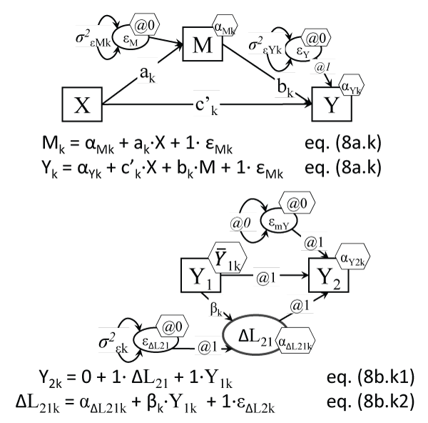
This particular analysis which combines mediation and FM has not been reported, to our knowledge, except in [47]. Such a model, shown in Figure 8a, can separate classes differing in any (or all) of the parameters estimated for a mediation (indirect effects) model: the direct, indirect, and total effects [48], as well as in the intercepts of the mediator and outcome, and possibly also in the primary cause->mediator (a) and the mediator-> outcome (b) coefficients, as shown in Figure 8a.
.
Figure 8a: The Mixture Mediation Model (MMM); the a,b,c notation
Notes: The a, b, & c' parameters can differ across classes k, as can the M and Y intercepts, and their residual variances; two other parameters cannot be easily shown in the model, the total effect (τ or TE) and the indirect effect (i or IE), which can also be expected to vary across classes k; another such parameter that could vary with k could be the correlation between εM and εY, which can be estimated only with additional instrumental variables.
Figure 8b: The Latent Change Mixture (LCM) model
Notes: A variant could be drawn like in Figure 7d; our notation makes evident what parameters can differ across classes k.
View Figure 8
Latent Change Mixture (LCM)
Another combination of continuous and categorical LVs is the LCS with unobserved classes [49], or what we call Latent Change Mixture (LCM) models (see Figure 8b). A better known (simpler) variant of the LCM is the Growth Mixture Model (GMM) [50], which assumes however only one global slope, and ignores subsequent pairwise changes. LCS with latent classes however can allow for differences between (unobserved) classes in any pairwise changes, as well as in proportional growth coefficients, and even in changes-to-changes coefficients.
Other Less Obvious Latent Variables
Some recent advances in statistical modeling brought to the forefront evidence for the latent (unknown, unobserved) nature of other statistical concepts. We briefly mention three of them here and provide visual depictions for one, but refer the readers to more detailed writings.
Latent class categorical LV with measurement error
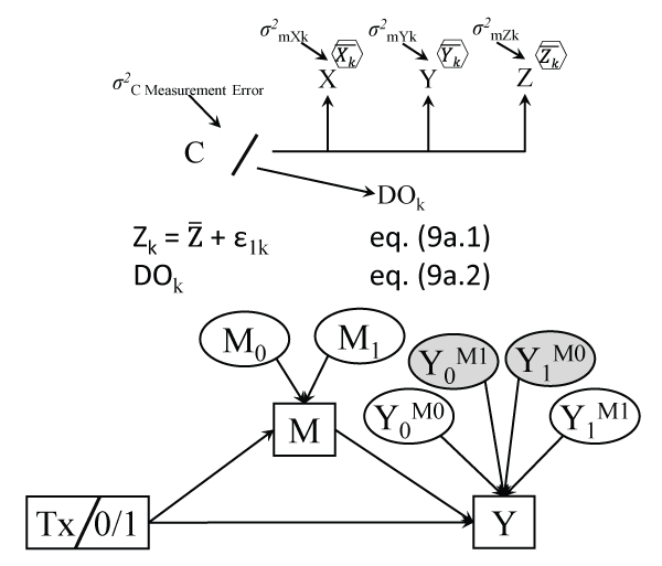
Models containing both Latent Class and latent regression analyses, in the family of Finite Mixture models (FM), like Growth Mixture Models (GMM) of distinct types of trajectories by latent classes of cases (people, patients, etc.), have pointed to the 'doubly latent' nature of the classification categorical latent variable C that represents the classes (class 1, 2, etc.). For example, in GMM models, the 'measurement model' component is meant to extract/uncover the classes using some indicators of the class latent variable (similar to indicators of a common factor in factor analysis [51]), while the 'predicting the class' part of the model allows for regressing this categorical C classification unto chosen predictors of class membership, yet a multi-class part of the model allows for 'effects' of the class variable unto distal outcomes [52]. Class variables however are estimated imperfectly, i.e. with measurement error, because each case gets estimated probabilities to belong to all classes, which are not clean-cut values like a 1.0 and the rest zeros, i.e. there is some mis-classification inherent in deciding that a case belongs to a single class (like error in classifying a person in terms of race/ethnicity). So there is measurement error contained in the C variable derived in statistical outputs, and hence the impact of it on a distal outcome is biased by this unreliability [23]; new methods have been developed recently to correct for such measurement error (e.g. the 3-step method [53]). Such a class latent variable then deserves two circles around it (see Figure 9a) in our opinion, one due to the inherent unknown nature of the latent class, the other from the measurement error it carries over once cases are assigned to classes [53].
.
Figure 9a: 'Doubly latent' variable in Latent Class Analysis
Notes: DO is a distal outcome; the 'regression' of DO on C represents in fact a number of pairwise contrasts between the means of DO (e.g. class 1 mean vs. last class mean, etc.). ; residual variances σ2 shown directly.
Figure 9b: Potential outcomes (POs) behind their observed counterparts
Notes: The relationships between the latent POs and their realizations M and Y are not testable causal relations; the treatment Tx has two conditions, 0 or control, and 1 or treated; the shaded 'latent' potential outcomes (POs) are fully unobservable or contrary-to-fact (CF, never accessible); Y0M1 means Y if all cases were not treated but their mediator attained its values, had cases been treated.
View Figure 9
Potential outcomes (PO)
In causal inference literature it is well known that estimating true causal effects, particularly the direct and indirect causal effects, requires reliance on variable values which have not been observed, called potential outcomes (PO), some of them which can never be observed by design, called contrary to fact (CF), or counterfactuals [54]. These can be seen as a form of LVs in fact, with half or all of their values not observed.
For example, when an intervention tries to reduce weight (outcome Y) by improving food habits (mediator M), the definition and estimation of causal indirect effects requires besides analyzing the observed M and Y variables their POs M0 and M1, or the mediator if all cases were not treated, or all were treated, respectively, and then also Y0M0, Y1M1 or: Y if all were not treated, but their mediator had values still under the not treated (control) condition (which we cannot observe for the treated cases of course), and Y if all were treated and their mediator was also that under treatment (unobserved for the control cases). The POs Y0M1 and Y1M0 are fully contrary-to-fact (CF), or inaccessible by researchers, and represent: Y if all were not treated but their mediator attained its values had all cases been treated, and finally Y if all were treated but their mediator reached values had they been in the control condition. While relationships between these 6 PO variables operating behind the 2 observed ones are not directly testable in linear causal models, assumptions behind the definition and estimation of causal indirect and direct effects refer to these POs rather than their observed counterparts [55]. Figure 9b is hence slightly misleading in fact, because once one estimates POs for the Y outcome e.g., total (and causal direct and indirect) effects can be directly computed for individual cases by mere subtraction [56], and for the entire sample by mere averaging: for example TEi = Y1M1i - Y0M0i, the pure direct effect dPi = Y1M0i - Y0M0i, and the total indirect effect iTi = Y1M1i - Y1M0i.
Dyadic LVs
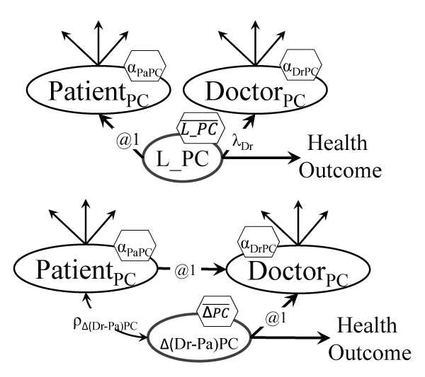
When a measure is captured from the members of a dyad like spouses, or patient and provider, such a concept needs to be modeled like a LV with indicators from each side of the dyad. Such a measure, like Patient Centeredness (PC [57]), needs to be linked to other predictors and outcomes from its LV form, rather than from the two separate (patient and doctor) observed PC components [58]. Such a dyadic model [21], like the one in Figure 10a, can yield a different effect on patients' health outcomes than a model with causal links from either the patients' or the doctors' component [59]. Other combinations of such paired (matched) variables are possible, like inserting LVs for the average or differences between the two components, much like a latent change score LCS model (shown earlier in Figure 5a), or a variety of actor-partner interdependence models (APIM [60]). The model in Figure 10b for instance would test whether larger discrepancies between patients and doctors' views of PC will affect patients' health outcomes.
.
Figure 10a: Dyadic model of patient centeredness (PC)
Notes: The mean of the true PC will differ from the means of patients' and doctors' views, and its effect on health outcomes will differ from the individual effects too.
Figure 10b: Dyadic model for doctor-patient discrepancy in views of patient centeredness (PC)
Notes: The patient and doctor PC are combined as ΔPC = (DoctorPC -PatientPC); an average could also be specified.
View Figure 10
Conclusion
The mission of statistics is to provide causal explanations that can be used to ultimately improve lives. The key ingredient in this endeavor is variability, since if we all were exactly the same there wouldn't be much to explain. The SEM-related visual statistical method we reviewed here approaches this task openly by referring to unexplained (co-)variability using double headed arrows, both for the variance of an exogenous variable (both arrows pointing towards that variable) and for the covariance between two variables: these quantities are not explained by the model, not yet at least. One goal of GLMM (and SEM) which has a clear visual analogue is to turn double headed arrows into single headed ones (or no link at all), and reduce unexplained variance, or to find causal explanations for observed variability and co-variability. Our visual graphical approach makes evident what is the target of the explanatory efforts and how one proposes the causal explanations, but also what assumptions are made in the process. We have shown in ten sets of displays that graphical causal models directly depicting latent variables (LVs) are common in most statistical analyses, and are valuable in better specifying model expectations and in separating out what is assumed (or known, therefore expected to be confirmed, i.e. the confirmatory part) from what needs to be estimated, or obtained, using data and the model assumptions (the exploratory part of the model). Such models can be used to completely describe statistical models in equation form, because they encode causal relationships that are directly translatable in regression form and even in matrix algebra [35]; they have an inherent obvious pedagogical value too. We chose for simplicity to focus on this translation and avoid complex GLMM (and SEM) details like estimation and fit.
We hope that by showing the link between visual graphs and testable statistical equations, and the ease of implementing such analyses based on explicitly modeling latent variables (LVs), these causal models will become more widespread in statistics practice, teaching and training.
Acknowledgements
The authors would like to thank the wider Active8 study team, including Holly Blake (Chief Investigator), Lucia Aguirre and Mark E. Batt. This work was supported by The BUPA Foundation (grant number: TBF-PPW11-018F).
Supplementary File
References
-
Chen B, J Pearl (2015) Graphical Tools for Linear Structural Equation Modeling. Forthcoming, Psychometrika.
-
Rabe-Hesketh S, Skrondal A (2008) Classical latent variable models for medical research. Stat Methods Med Res 17: 5-32.
-
Rabe-Hesketh S, A Skrondal, A Pickles (2004) Generalized multilevel structural equation modeling. Psychometrika 69: 167-190.
-
Skrondal A, S Rabe-Hesketh (2004) Generalized latent variable modeling: Multilevel, longitudinal, and structural equation models. Chapman & Hall/CRC.
-
Wright S (1921) Correlation and causation. Part I Method of path coefficients. Journal of agricultural research 20: 557-585.
-
Muthén BO (2002) Beyond SEM: General latent variable modeling. Behaviormetrika. 29: 81-118.
-
Kline R (2010) Principles and Practice of Structural Equation Modeling. (3rd edn), The Guilford Press.
-
Hayduk LA (1987) Structural equation modeling with LISREL: Essentials and advances. Johns Hopkins University Press.
-
Wang C-P, B Jo, C Hendricks Brown (2014) Causal inference in longitudinal comparative effectiveness studies with repeated measures of a continuous intermediate variable. Stat Med 33: 3509-3527.
-
Pearl J (2013) Structural counterfactuals: a brief introduction. Cogn Sci 37: 977-985.
-
ftp://ftp.cs.ucla.edu/pub/stat_ser/r439.pdf
-
Pearl J (1998) Graphs, causality, and structural equation models. Sociological Methods & Research 27: 226.
-
Pearl J (2009) Causality: models, reasoning, and inference. (2nd edn), Cambridge university press Newyork, USA.
-
Pearl J (2011) The structural theory of causation. In: Phyllis McKay Illari, Federica Russo, Jon Williamson Causality in the Sciences. Oxford Scholarship.
-
Muthén LK, BO Muthén (1998-2012) Mplus User's Guide. (7th edn), Los Angeles, CA: Muthén & Muthén.
-
Bollen KA (2002) Latent variables in psychology and the social sciences. Annu Rev Psychol 53: 605-634.
-
Arbuckle J (2007) Amos (Version 5.0) [Computer Program]. Chicago: SPSS.
-
Muthén LK, BO Muthén (2002) How to use a Monte Carlo study to decide on sample size and determine power. Structural Equation Modeling 9: 599-620.
-
Wright S (1934) The Method of Path Coefficients. The Annals of Mathematical Statistics 5: 161-215.
-
McArdle JJ, F Hamagami (2001) Latent difference score structural models for linear dynamic analyses with incomplete longitudinal data. In: L. Collins, New methods for the analysis of change: Decade of behavior. Washington, DC, 139-175.
-
Kenny D, D Kashy, W Cook (2006) Dyadic data analysis. The Guilford Press.
-
McArdle JJ, F Hamagami (2006) Longitudinal tests of dynamic hypotheses on intellectual abilities measured over sixty years. In: C.S. Bergeman and S.M. Boker, Methodological Issues in Aging Research. Lawrence Erlbaum Associates: Mahwah, NJ.
-
Bollen KA (1989) Structural equations with latent variables. John Wiley and Sons.
-
Kelley TL (1942) The reliability coefficient. Psychometrika 7: 75-83.
-
Wainer H (2001) Augmented scores-"borrowing strength" to compute scores based on small numbers of items. In: D. Thissen and H. Wainer, Test scoring. Lawrence Erlbaum, Mahwah, NJ.
-
Blake H (2015) Active8! Technology-based intervention to promote physical activity in hospital employees. American Journal of Health Promotion.
-
Coman EN, Eugen Iordache, Lisa Dierker, Judith Fifield, Jean J. Schensul (2014) Statistical power of alternative structural models for comparative effectiveness research: advantages of modeling unreliability. Journal of Modern Applied Statistical Methods 13: 71-90.
-
Trafimow D (2014) Estimating true standard deviations. Front Psychol 5: 235.
-
Cohen J (1968) Multiple regression as a general data-analytic system. Psychological Bulletin. 70: 426-443.
-
Orzechowski KM, Nicholas SS, Baxter JK, Weiner S, Berghella V (2014) Implementation of a universal cervical length screening program for the prevention of preterm birth. Am J Perinatol 31: 1057-1062.
-
Coman EN, Picho K, McArdle JJ, Villagra V, Dierker L, et al. (2013) The paired t-test as a simple latent change score model. Front Psychol 4: 738.
-
Voelkle MC (2007) Latent growth curve modeling as an integrative approach to the analysis of change. Psychology Science. 49: 375-414.
-
Duncan T, S Duncan, L. Strycker (2006) An Introduction to Latent Variable Growth Curve Modeling: Concepts, Issues, and Applications. (2nd edn), Lawrence Erlbaum Associates, Mahwah, N.J.
-
Kline RB (2011) Convergence of Structural Equation Modeling and Multilevel Modeling. In: M. Williams and W.P. Vogt, The SAGE Handbook of Innovation in Social Research Methods. Sage Publications Ltd.
-
McArdle JJ (2009) Latent variable modeling of differences and changes with longitudinal data. Annu Rev Psychol 60: 577-605.
-
Malone PS, Lansford JE, Castellino DR, Berlin LJ, Dodge KA, et al. (2004) Divorce and Child Behavior Problems: Applying Latent Change Score Models to Life Event Data. Struct Equ Modeling 11: 401-423.
-
Grimm KJ, Yang An, John J McArdle, Alan B, Zonderman, et al. (2012) Recent Changes Leading to Subsequent Changes: Extensions of Multivariate Latent Difference Score Models. Structural Equation Modeling: A Multidisciplinary Journal 19: 268-292.
-
Coman EN, Carolyn A Lin, Suzanne L Suggs, Eugen Iordache, John J McArdle, et al. (2014) Altering dynamic pathways to reduce substance use among youth: Changes achieved by dynamic coupling. Addiction Research & Theory 22: 505-514.
-
Enders CK (2010) Applied missing data analysis. (1st edn), Guilford Publications.
-
Graham JM (2008) The General Linear Model as Structural Equation Modeling. Journal of Educational and Behavioral Statistics 33: 485-506.
-
Petter S, D Straub, A Rai (2007) Specifying formative constructs in information systems research. Mis Quarterly 31: 623-656.
-
Saris WE, IN Gallhofer (2007) Design, Evaluation, and Analysis of Questionnaires for Survey Research. John Wiley & Sons, Newbury Park, CA.
-
Coman EN, Iordache E, Schensul JJ, Coiculescu I (2013) Comparisons of CES-D depression scoring methods in two older adults ethnic groups. The emergence of an ethnic-specific brief three-item CES-D scale. Int J Geriatr Psychiatry 28: 424-432.
-
Muthén B, Shedden K (1999) Finite mixture modeling with mixture outcomes using the EM algorithm. Biometrics 55: 463-469.
-
Lubke GH, Muthén B (2005) Investigating population heterogeneity with factor mixture models. Psychol Methods 10: 21-39.
-
Kuo P-H, Steven H Aggen, Carol A Prescott, Kenneth S Kendler, Michael C. Neale, et al. (2008) Using a factor mixture modeling approach in alcohol dependence in a general population sample. Drug and alcohol dependence 98: 105-114.
-
Coman E, Judith Fifield, Suzanne Suggs, Deborah Dauser-Forrest, Martin-Peele Melanie (2014) Probing causal mechanisms and strengthening causal inference by means of mixture mediation modeling. Modern Modeling Methods Conference, Session 3.5: Modeling Treatment and Causal Effects, Storrs, CT.
-
Baron RM, DA Kenny (1986) The moderator-mediator variable distinction in social psychological research: Conceptual, strategic, and statistical considerations. J Pers Soc Psychol 51: 1173-1182.
-
McArdle JJ, KJ Grimm (2010) Five Steps in Latent Curve and Latent Change Score Modeling with Longitudinal Data. Longitudinal research with latent variables 245-273.
-
Muthén BO (2001) Second-generation structural equation modeling with a combination of categorical and continuous latent variables: New opportunities for latent class/latent growth modeling. In: A. Sayer and L. Collins, New methods for the analysis of change. American Psychological Association, Washington DC, 291-322.
-
Asparouhov T, B Muthén (2014) Auxiliary variables in mixture modeling: 3-step approaches using Mplus. Mplus Web Notes: No. 15.
-
Nylund-Gibson K, Ryan Grimm, Matt Quirk, Michael Furlong (2014) A Latent Transition Mixture Model Using the Three-Step Specification. Structural Equation Modeling: A Multidisciplinary Journal 21: 439-454.
-
Asparouhov T, B Muthén (2014) Auxiliary Variables in Mixture Modeling: Three-Step Approaches Using Mplus. Structural Equation Modeling: A Multidisciplinary Journal 21: 329-341.
-
Pearl J (2010) An introduction to causal inference. Int J Biostat 6: Article 7.
-
Jo B (2008) Causal inference in randomized experiments with mediational processes. Psychol Methods 13: 314-336.
-
Coman EN (2015) How to use causal mediation tools to make patient-centered decisions for maximized individual benefit. International Journal of Person Centered Medicine.
-
Mead N, Bower P (2000) Patient-centredness: a conceptual framework and review of the empirical literature. Soc Sci Med 51: 1087-1110.
-
Coman E (2014) Patient Centeredness. Modern Approaches Using Dyadic Research: Implications for Providers. CIPCI-TRIPP Roundtable - The Connecticut Institute for Primary Care Innovation & Ethel Donaghue Center for Translating Research into Practice and Policy, Hartford, CT.
-
Kenny DA, Lawrence, La Voie (1985) Separating Individual and Group Effects. Journal of Personality & Social Psychology 48: 339-348.
-
Kenny DA (1996) Models of Non-Independence in Dyadic Research. Journal of Social and Personal Relationships 13: 279-294.


