The Coronavirus Disease 2019 (COVID-19) has posed a great threat to global public health; of which was reported to emerge in Wuhan, China at the end of the year 2019. It became alarming to Nigerians when Nigeria recorded her first index case in February 2020 in the city of Lagos which has led to a total number of 5162 confirmed cases, 1180 recovered with 167 death recorded as at May 14, 2020. This paper proposes a mathematical model SEIQCRW which adopt the SEIR model to study the current outbreak of COVID-19 in Nigeria with nonlinear forces of infection. This model defines the transmission channels in the infection dynamics and the impact of the environmental reservoir in the transmission and spread of this disease to humans. The existence of the region where the model is epidemiologically feasible is established. A detailed numerical simulation of this model was conducted using the Nigeria Centre for Disease Control (NCDC) reported data. Our analytical and simulation results between February 29, 2020 and May 14, 2020 are in good agreement. Further simulation indicates that Nigeria's cumulative number of confirmed cases will reach 55,000 individuals in December 25, 2020. Mitigation strategies and its effectiveness in reducing the spread of COVID-19 across Nigeria are considered.
COVID-19, Infection dynamics, Mathematical model, SEIQCRW model, Transmission, Basic reproduction number, Nigeria
The Coronavirus Disease 2019 (COVID-19) formerly known as a novel coronavirus (2019-nCoV) caused by severe acute respiratory syndrome coronavirus 2 (SARS-CoV-2) is highly transmissible [1,2] and has posed a great threat to the global public health, of which was reported by the World Health Organization (WHO) to emerged in Wuhan City, Hubei province of China at the end of the year 2019. The Federal Ministry of Health confirmed Nigeria's first index case in Lagos State, Nigeria, on the 27th of February, 2020, since the beginning of the outbreak in China. The first case was an Italian citizen, who works in Nigeria and returned from Milan, Italy to Lagos, Nigeria on the 25th of February, 2020. The second case was found in Ewekoro, Ogun State, Nigeria, where the patient was reported to have had contact with the Italian man [3]. And from there it has spread across to all States in Nigeria and had led to a total number of 5162 confirmed cases as at May 14, 2020. Which can be traced to the fact that the asymptomatic infected individuals show no symptoms, making it easy to infect other individuals with close contact often in an unconscious manner in crowded places like markets. Thus, increasing the concentration of the virus in the environmental reservoir as these viruses can stay up to some days in the environment thereby increasing the risk of infection through surface and fomites [4]. In a bid to combat the spread of the COVID-19 pandemic, the Federal government imposed lockdown measures in the three States of Lagos, Abuja-FCT and Ogun, other States received an inflow of people from these States without prior isolation and testing of travelers. This has also been attributed to the spread of coronavirus to other States that hitherto had zero infected case. The Nigeria Centre for Disease Control (NCDC) has targeted the testing of about two million people in the next three (3) months of May to July, 2020 (NCDC, 2020). In a bid to increase the number of testing capacities in the country's huge population of over 200 million people, the NCDC has expanded the testing laboratories across the country to 18. As the country continues to roll out mitigation strategies to flatten the curve and reduce the spread of the virus across communities and States, some people are of the opinion that Coronavirus is a myth.
Due to the exponential spread of COVID-19 in Nigeria, the need to develop a mathematical model to study the dynamics of the transmission and the spread of this infectious diseases capturing the quarantined individuals, the confirmed cases and the concentration of these pathogens in the environmental reservoir.
Several modelling studies have been done to analyze the spread of COVID-19 pandemic, ranging from stochastic modelling [5,6] to mathematical modelling [7-10]. In [9], SEIRU model involving the susceptible, the exposed, the infected, the quarantined and the recovered individuals were considered. It was predicted that there is a chance of a decline in secondary infections when all precautionary measures are observed globally. In [7], a mathematical model was developed to describe a Bat-Hosts-Reservoir-People transmission network model for simulating the potential transmission from infection source to human, which was simplified to Reservoir-People transmission network model. The reproduction number was calculated from the Reservoir-People model using the next-generation matrix to measure the transmissibility of the virus in Wuhan, China. The value of was estimated to be 2.30 from the environmental reservoir to humans and 3.58 from humans to humans. In [10], a compartmental model involving the susceptible, the exposed, the infected, the recovered and the concentration of the pathogen in the environmental reservoir was considered. The reproduction number was calculated using the next-generation matrix to determine the transmissibility of the virus from the exposed, the infected and the pathogens in the environmental reservoir to the susceptible in Wuhan, China. The value of was estimated to be 4.25 covering 1.5 from indirect transmission route and 2.7 from direct transmission route.
However, model considering the quarantined individuals, confirmed cases, nonlinear forces of infection in the form of saturated incidence rates in humans and the impact of the indirect transmission route from the virus in the environmental reservoir to humans were not considered in the published models. Hence, we present a mathematical model for the pandemic COVID-19 to describe the several transmission pathways including the disease-induced rates for humans, nonlinear forces of infection in the form of saturated incidence rates in humans, direct and indirect transmission routes. The direct transmission routes describe the transmission from the exposed individuals to the susceptible individuals and from the infected individuals to the susceptible individuals, while the indirect transmission routes come from the interaction of the susceptible individuals with these pathogens in the environmental reservoir.
To study the transmission and the spread of COVID-19 among human, we formulate a model which divides the total population of human at time t into six components. The Susceptible population denoted by S, the Exposed population denoted by E, the Infected population denoted by I, the Quarantined population denoted by Q, the Confirmed cases denoted by C, and the Recovered population denoted by R. This study adopt the SEIR model framework with total population of human of size N with additional classes, the Quarantined (Q) and the Confirmed cases (C).
The susceptible population are individuals who may be infected with the virus, the exposed population are individuals who have been infected but they are without symptoms usually at the early stage or incubation period of the virus. The infected population are those that are fully showing the disease symptoms usually the latent period of the virus and are capable of infecting others. The exposed population E and the infected population I contains asymptomatic infected and symptomatic infected individuals respectively. The quarantined population Q are individuals who are quarantined for some time, if they start showing symptoms of the infectious disease and are tested to determine whether the diagnosis is confirmed C. If tested positive to the virus, they are isolated to receive treatment. After a period of treatment and have satisfied all observatory requirement, they moved to the recovered population R.
The compartmental model which shows the mode of transmission of COVID-19 is depicted in the Figure 1 and Figure 2.
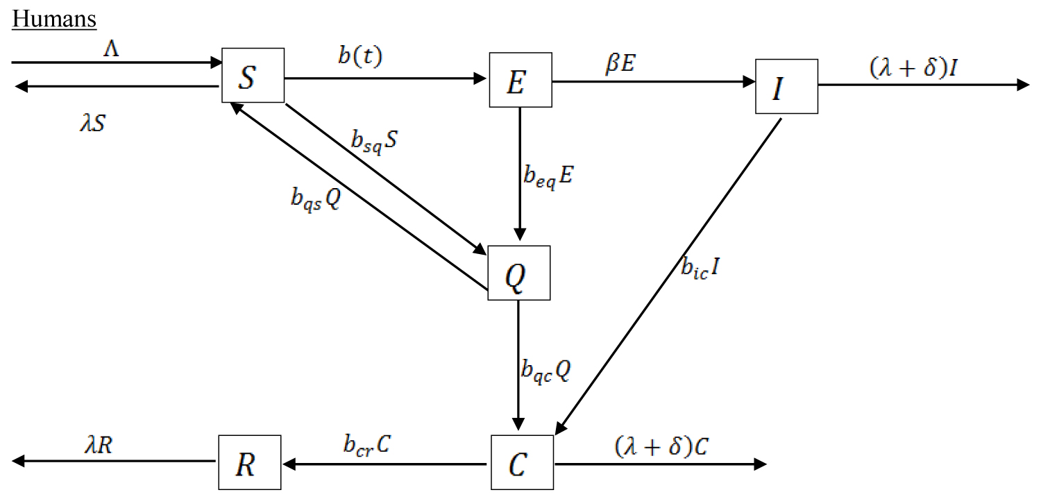 Figure 1: Compartmental transmission of COVID-19 among Humans.
View Figure 1
Figure 1: Compartmental transmission of COVID-19 among Humans.
View Figure 1
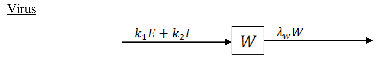 Figure 2: Compartmental concentration of the virus in the environmental reservoir.
View Figure 2
Figure 2: Compartmental concentration of the virus in the environmental reservoir.
View Figure 2
The parameters used for the transmission model are described in the Table 1.
Table 1: Symbols, value and source of parameters used in the model. View Table 1
Number of Individuals susceptible to infection at a given time t
Number of individuals infected but without symptoms at a given time t
Number of individuals infected but not yet isolated at a given time t
Number of individuals quarantine at a given time t
Number of individuals confirmed to be infected with the virus, isolated and expecting recovery at time t
Number of individuals recovered at time t
From the compartmental model, we obtain a seven-dimensional system of ordinary differential equation which describes the dynamic transmission mechanism of the infectious disease as:
Together with the initial conditions
Where W is the concentration of the virus in the environmental reservoir. The parameter represent the population influx, λ is the natural death in human, δ is the disease-induced fatality rate, is the incubation period between the infected and the onset of symptoms, is the rate of recovery from the infectious disease. is the rate at which those that are fully showing the disease symptoms are diagnosed to be positive to the disease. We assume that not all individuals showing the disease symptoms are infected with COVID-19 because Influenza is also a respiratory disease with related symptoms as COVID-19 which can also be transmitted by contacts droplet and fomites [11]. is the rate at which individual are quarantined being traced to have had contact with those confirmed to be positive. If they do not show symptoms, they are removed back to the susceptible population at the rate of . is the rate at which individuals from the exposed population are quarantined, is the rate at which quarantined individuals are diagnosed to be positive to the disease. are the rates of the exposed and infected human contributing the infectious disease to the environmental reservoir and is the removal of the virus from the environment due to some control measure. is the infection degree of the infectious disease in the susceptible population, the mathematical expression is as follows:
The function respectively denotes the direct (human-to-human) transmission rate between susceptible population and the exposed population and between susceptible population and the infected population and the infected population respectively. The denotes the indirect (environment to human) transmission rate. is further defined as:
Where are positive constants representing the maximum values of these transmission rates and is a positive coefficient (otherwise constant) providing adjustment to the transmission rate.
Some of the parameters estimate used for simulation of this work are available in the literature. Others are estimated from the available COVID-19 data (confirmed cases, recovered cases, deaths, and samples tested) published by the NCDC [12] to stimulate the unknown parameters. Population and birth rate data were collected from [13]. The initial data correspond to the epidemic data officially released on 29th of February, 2020. The corresponding estimated parameters are obtained by fitting an optimization method (Maximum Likelihood Estimation (MLE)) based on the reported data and the epidemic occurrence is predicted for the future. This is analyze using Python 3.6 by generating a curve fitting model using scipy.stats library with optimize option and passing some initial guesses for the parameters, which are fitted with numpy. The maximum likelihood estimation allows the determination of parameter sets by maximizing the likelihood that the process described by the model produced the reported data on NCDC website. We fit the cumulative number of confirmed cases generated from the model (1.1) to the NCDC reported data of cumulative number of confirmed cases, which are in agreement with the reported data from February 29, 2020 to May 14, 2020 (Figure 3).
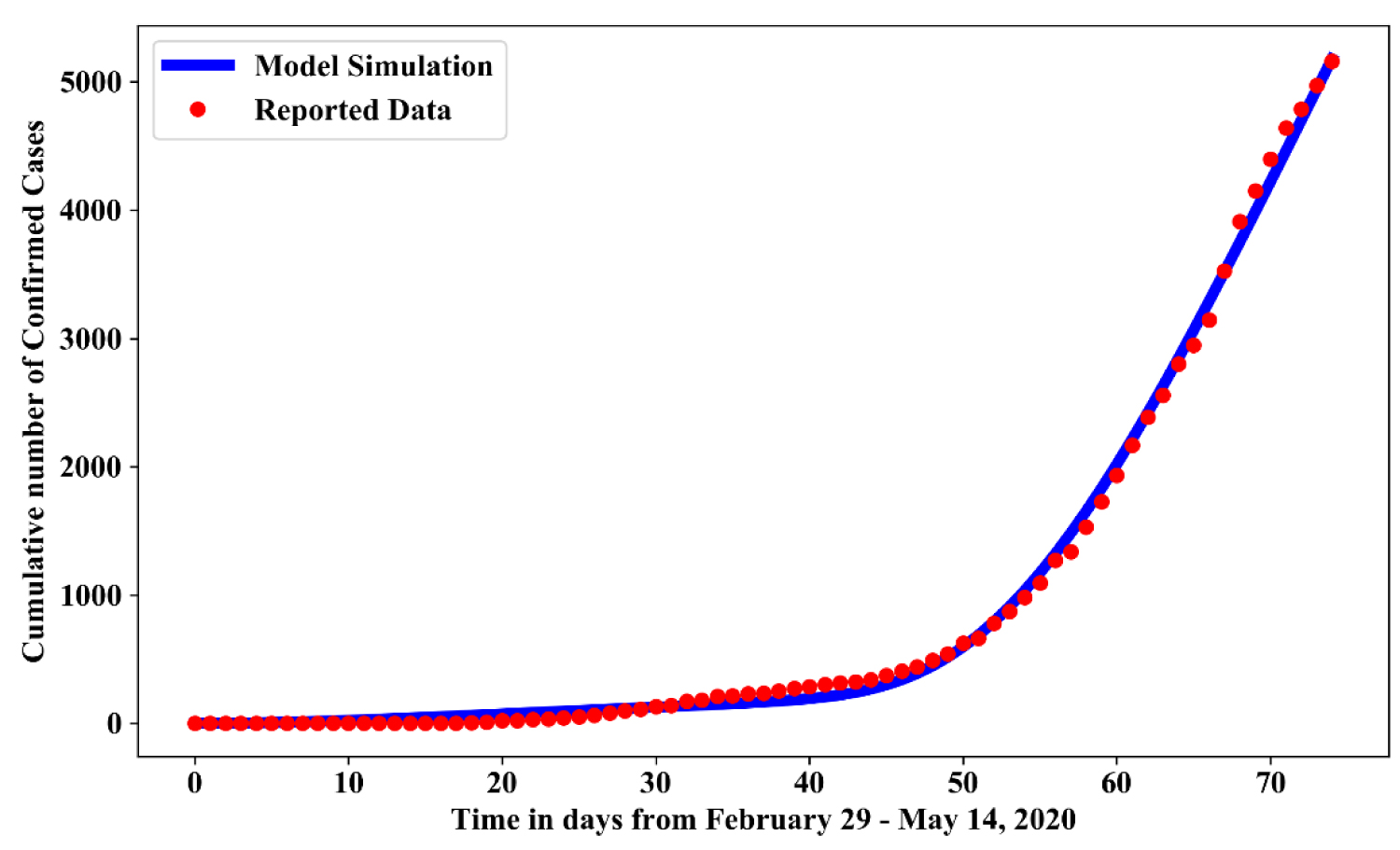 Figure 3: Simulation showing model simulated data and reported data of confirmed cases.
View Figure 3
Figure 3: Simulation showing model simulated data and reported data of confirmed cases.
View Figure 3
The following provides the result which guarantees the dynamic transmission governed by the system (1.1) is epidemiologically and mathematically well-posed in a feasible region given by
and
Since,
Theorem 1: There exist a domain in which the solution set is contained and bounded.
Proof: Following the idea of [14]
Given the solution set with positive initial conditions (1.2), we let
and
Then the time derivatives along solutions of the system (1.1) are obtained by
and
It follows that
Solving the differential equations (1.3) yield
and
Consequently, taking the limits as yields
Thus, all solutions of the population are confined in the feasible region , showing that the feasible region for the formulated model in the equation (1.1) exist and is defined by
Here, we state the result of the disease-free and endemic equilibrium of the model. The point at which the differential equation of the system (1.1) equals to zero is the equilibrium point. It should be noted that as long the growth term is not equal to zero, there will be no trivial equilibrium point. Consequently, and the population will not vanish.
Existence of disease-free equilibrium point: Disease-free equilibrium points are steady-state solutions or equilibrium point where there's no infection of COVID-19. Thus, at the disease-free equilibrium point , we have that . Hence, the resulting disease-free equilibrium point obtained solving (1.1) is
Basic reproduction number: Reproduction number is an important topic in epidemiological models which is usually denoted by . It is an important parameter that predicts whether an infection will spread throughout the population or not.
To obtain for the model in (1.1), we use the next generation matrix technique [15,16]. The infection component in this model are . Finding the derivatives at the disease-free equilibrium point. The infection matrix and the transition matrix are respectively
Where,
The basic reproduction number of model (1.1) is defined as the spectral radius of the product . Hence, the reproduction number for the model (1.1) is
The first two parts of in (1.5) i.e. and measures the contribution from human to human transmission routes (exposed to susceptible, infected to susceptible respectively) and the third par measures the contribution from the environment to human transmission route. These three transmission modes encapsulate the overall infection risk for the outbreak of COVID-19.
Theorem 2: The disease-free state is asymptotically stable if and unstable if
Proof: The Jacobian matrix of the system (1.1) at the disease-free equilibrium point is obtained as
Where, and
We need to show that the eigenvalue of are all negative. The sixth column and the second row contains only the diagonal entry which forms two negative eigenvalues , the other five eigenvalues can be obtained from the sub-matrix formed by excluding the sixth row and column and the second row and column. Hence, we have
In the same way, the second row and the fourth column contains the diagonal terms which form a negative eigenvalue . The remaining three eigenvalues are obtained from the sub-matrix
Furthermore, the last row contains the diagonal terms which form a negative eigenvalue . The remaining two eigenvalues are obtained from the sub-matrix
The eigen values of the matrix are the root of the characteristics equation
With the roots
So that
and
is a negative eigenvalue and is a negative eigenvalue if . Hence, all the eigenvalues of are negative which imply the disease-free point is asymptotically stable. Thus for a free state to occur the product of the rate of removal from quarantined and susceptible population must be greater than the product of the rate of entering from susceptible to quarantined and from quarantined population back to the susceptible population.
But if , it implies that there is one eigenvalue with positive real part and the disease-free equilibrium (DFE) point is unstable.
Here, we shall show that the formulated model (1.1) has an endemic equilibrium point E1
Theorem 3: The model (1.1) has no endemic equilibrium when and a unique endemic equilibrium exist when
Proof: Let be a nontrivial equilibrium of the model (1.1), setting the differential equation in model (1.1) to zero, we have
Where
And is a positive solution of an equation given by
With
From (1.6), for , when , we have that which implies that by Routh-Hurwitz criterion [17], the model (1.1) has no positive solution. However, when , then and endemic equilibrium exists.
In this study, we proposed SEIQCDRW transmission model, which considered the routes from the environment to human and from human to human. We considered the prevalence of COVID-19 in Nigeria using model (1.1). The simulation result showed that the is 2.68 specifically, we have that
Which quantify the infection risk from each of the transmission routes. being the largest comes from the exposed to susceptible transmission, since those exposed shows no symptoms, making it easy to shed the virus to other individuals with close contact often in an unconscious manner majorly in public places. The smallest component comes from the infected to susceptible, which can be traced to the body being down and would not be able to move around unlike the exposed. From our simulation, the basic reproduction number for humans in Nigeria is 2.25. Lastly, shows the contribution of the virus from the environment to human.
As earlier mentioned, the parameters used were fitted using maximum likelihood estimation and optimization package in Python 3.6. The parameters used in this work are tabulated in Table 1
This involves reducing the transmission rate/contact rate from the exposed to susceptible, highly infectious to susceptible and environment to human. The effect of social distancing can be monitored by simulating the model using the estimated parameters in Table 1 with the following effective measure of social distancing:
(i) Slight level of effectiveness of social distancing: This requires reducing the transmission rates by 15% such that we have = 2.861e-7 and = 5.437e-8
(ii) Average level effectiveness of social distancing: This requires reducing the transmission rates by 50% such that we have = 1.683e-7 and = 3.198e-8
(iii) Strict level effectiveness of social distancing: This requires reducing the transmission rates by 75% such that we have = 8.415e-8 and = 1.599e-8
Figure 4 shows the simulation for various effectiveness of social-distancing control measures in the absence of hygienic culture and face mask. For no social-distancing measured as the base line value estimated in Table 1, while, slight social distancing, average social distancing and strict social distancing measured as 15%, 50% and 75% reduction of their baseline value respectively. In comparison with no social distancing, result shows that: adopting a strict social distancing will reduce the cumulative number of confirmed cases by 54%-58%; adopting average social distancing will reduce the cumulative number of confirmed cases by 41%-45% while adopting slight social distancing will the cumulative number of confirmed cases by 23%-27%. Increasing social-distancing control measure would results in reduction in the number of individuals that would be confirmed with COVID-19.
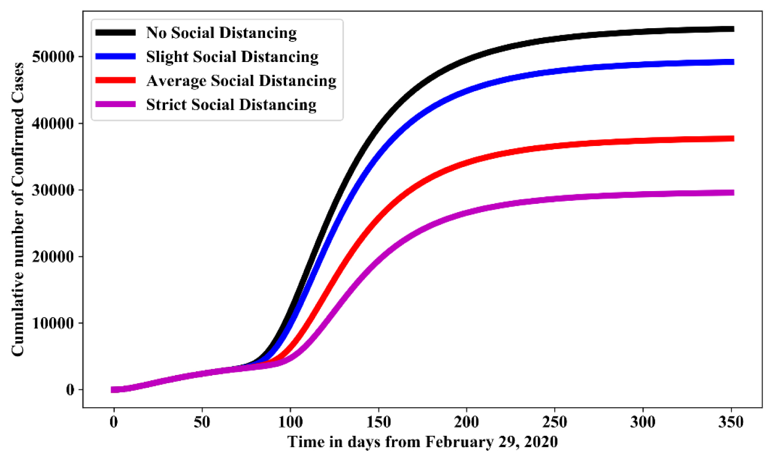 Figure 4: Simulation of model (1.1) for various effectiveness of social-distancing control measures in the absence of hygienic culture and face mask.
View Figure 4
Figure 4: Simulation of model (1.1) for various effectiveness of social-distancing control measures in the absence of hygienic culture and face mask.
View Figure 4
This involves increasing the transmission rate/contact rate from the exposed to susceptible, highly infectious to susceptible and environment to human. The effect of relaxation of lockdown can be monitored by simulating the model using the estimated parameters in Table 1 with the following effective measure of social distancing: culture
(i) Slight relaxation of lockdown measures: This requires reducing the transmission rates by 15% such that we have = 3.871e-7 and = 7.355e-8
(ii) Average relaxation of lockdown measures: This requires reducing the transmission rates by 50% such that we have = 5.049e-7 and = 9.594e-8
(iii) Full relaxation of lockdown measures: This requires reducing the transmission rates by 75% such that we have = 5.891e-7 and = 1.119e-7
Figure 5 shows the simulation for various level of relaxation of lockdown control measures in the absence of hygienic culture and face mask. For no relaxation of lockdown measured as the baseline value in Table 1, while, slight relaxation of lockdown, average social relaxation of lockdown and strict relaxation of lockdown measured as 15%, 50% and 75% increase of their baseline value respectively. In comparison with no relaxation of lockdown, result shows that: full relaxation of lockdown increases the cumulative number of confirmed cases by 66%-68%; average relaxation of lockdown increases the cumulative number of confirmed cases by 33%-35%; slight relaxation of lockdown increases the cumulative number of confirmed cases by 11%-13%.
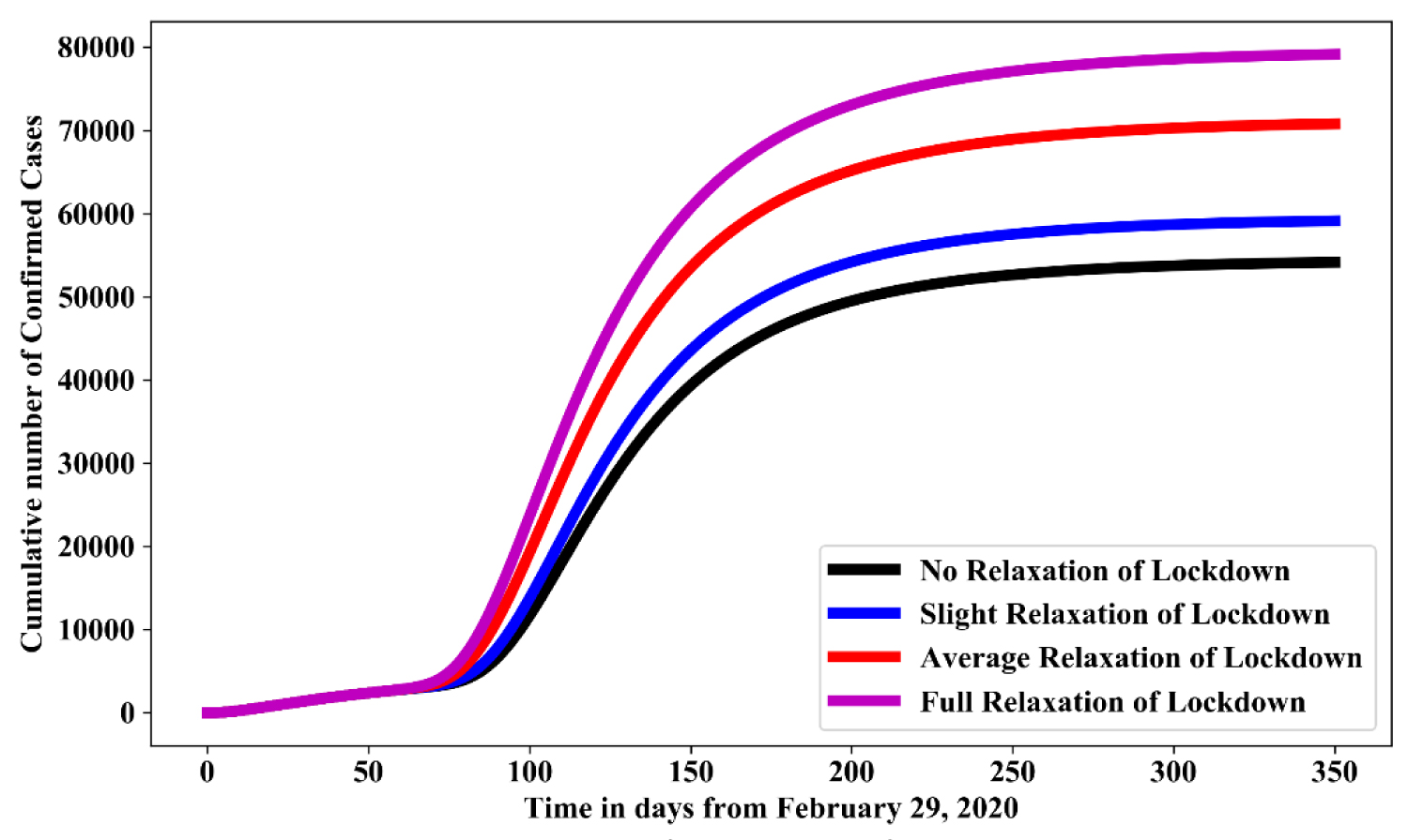 Figure 5: Simulation of model (1.1) for various level of relaxation of lockdown control measures in the absence of hygienic culture and face mask.
View Figure 5
Figure 5: Simulation of model (1.1) for various level of relaxation of lockdown control measures in the absence of hygienic culture and face mask.
View Figure 5
This involves decreasing the transmission rate/contact rate from environment to human. The effect of maintaining a hygienic culture (fumigation of the environment and hand washing) can be monitored by simulating the model using the estimated parameters in Table 1 with the following effective measures:
(i) Slight hygienic culture measures: This requires reducing the transmission rates from the environmental reservoir to the susceptible class () by 15% such that we have () = 1.6031e-7
(ii) Average hygienic culture measures: This requires reducing the transmission rates from the environmental reservoir to the susceptible class () by 50% such that we have = 9.43e-8
(iii) Full hygienic culture measures: This requires reducing the transmission rates from the environmental reservoir to the susceptible class () by 75% such that we have = 4.71e-8
Figure 6 shows the simulation for various level of hygienic culture in the absence of social distancing and face mask. For no hygienic culture is measured as the baseline value in Table 1, while, slight hygienic culture, average social hygienic culture and strict hygienic culture measured as 15%, 50% and 75% increase of their baseline value respectively. In comparison with no hygienic culture, result shows that: strict hygiene culture reduces the cumulative number of confirmed cases by 40%-45%; average hygienic culture reduces the cumulative number of confirmed cases by 30%-35%; while slight hygienic culture reduces cumulative number of confirmed cases by 10%-15%.
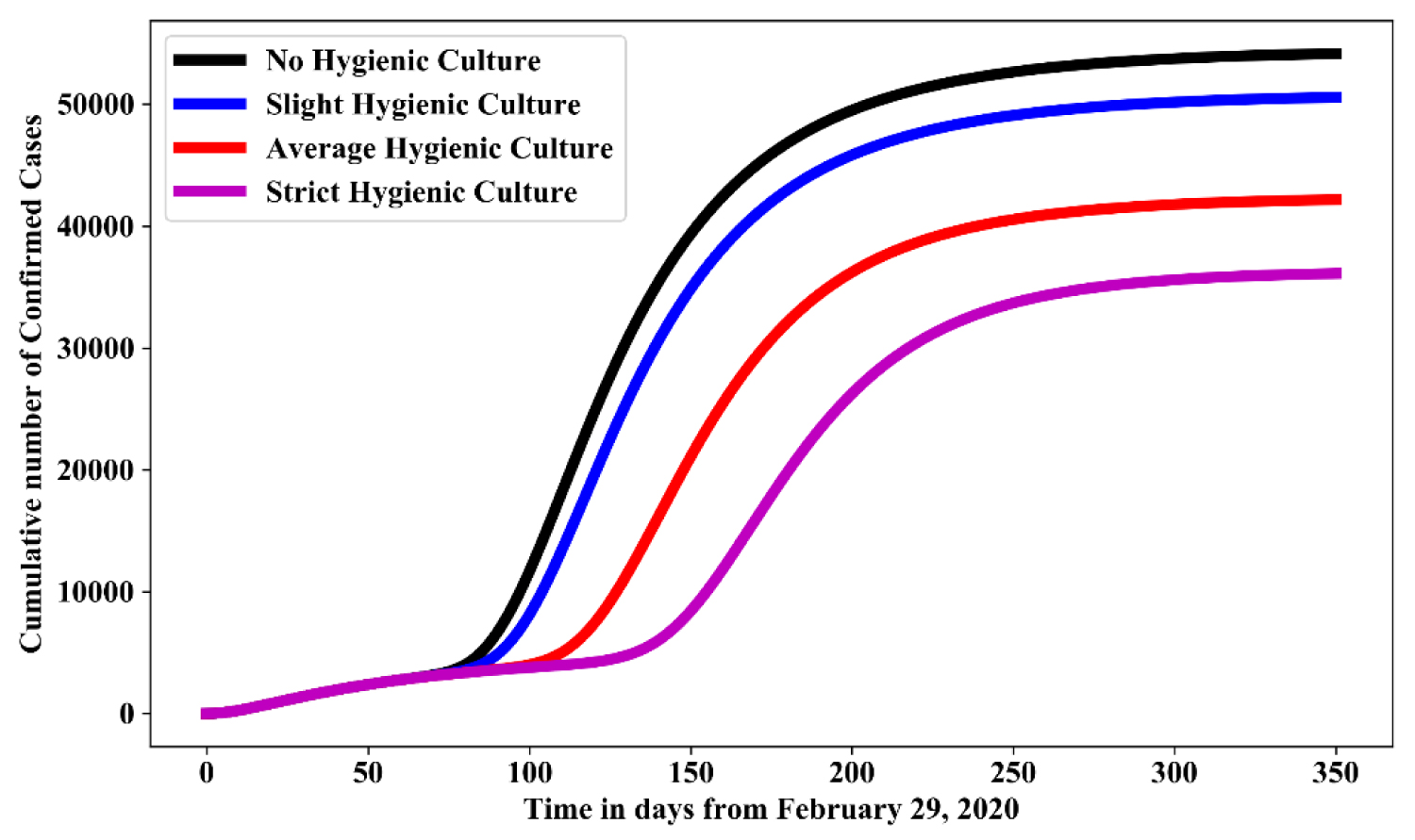 Figure 6: Simulation of model (1.1) for various effectiveness of hygienic culture control measures in the absence of face mask and social-distancing.
View Figure 6
Figure 6: Simulation of model (1.1) for various effectiveness of hygienic culture control measures in the absence of face mask and social-distancing.
View Figure 6
This involves increasing the adjustment control coefficient to the transmission rate/contact rate from the exposed to susceptible, highly infectious to susceptible and environment to human with the use of face masks. In order to provide adjustment to the number of individuals infected, we increase , the adjustment coefficient providing adjustment to the number of individuals exposed and infected. From the estimated parameter in Table 1.
Figure 7 shows the simulation for various effectiveness of face mask control measure in the absence of social distancing and hygienic culture. For Usage of facemask is measured as the baseline value in Table 1. In comparison with no usage of face mask, result shows that: 25% usage of face mask will reduce the cumulative number of confirmed cases by 45%-50%; 50% usage of face mask will reduces the cumulative number of confirmed cases by 70%-75%; while 75% usage of face mask reduces cumulative number of confirmed cases by 80%-85%.
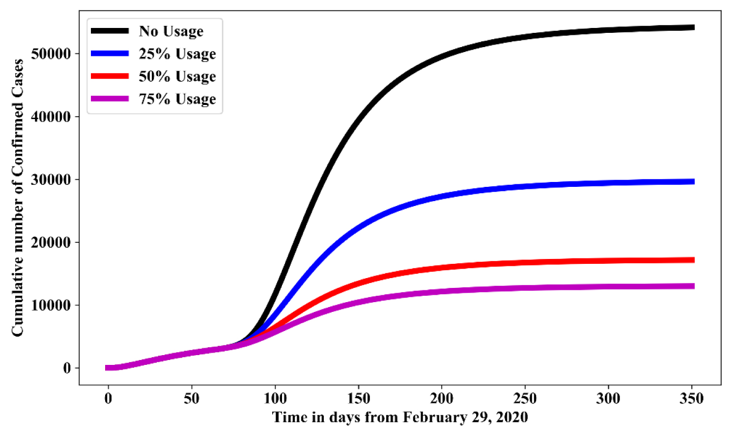 Figure 7: Simulation of model (1.1) for various effectiveness use of face mask control measure in the absence of social-distancing and hygienic culture.
View Figure 7
Figure 7: Simulation of model (1.1) for various effectiveness use of face mask control measure in the absence of social-distancing and hygienic culture.
View Figure 7
In order to consider the effect of complying will the assessment control mentioned earlier, we consider 75% compliance with the use of facemask and maintaining full hygienic environment along with relaxation of lockdown as follows:
(a) Full relaxation of lockdown with 75% effective use of Face Mask and Full hygienic cultural measure
(b) Average relaxation of lockdown with 75% effective use of Face Mask and Full hygienic cultural measure
Figure 8 and Figure 9 shows the simulation for 75% effective use of face mask, full hygienic culture with average relaxation and full relaxation respectively. In the presence of 75% effective use of face mask and maintaining strict hygienic culture will reduce the cumulative confirmed cases by 78%-80% and 73%-75% respectively.
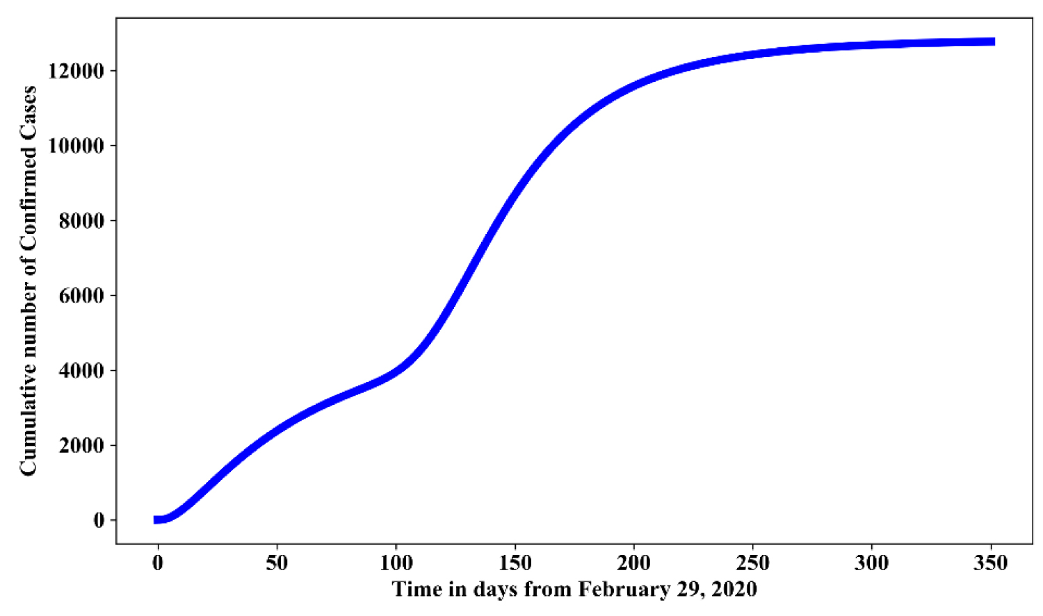 Figure 8: Simulation of model (1.1) for an average relaxation of lock down with 75% effective use of face mask and strict hygienic culture.
View Figure 8
Figure 8: Simulation of model (1.1) for an average relaxation of lock down with 75% effective use of face mask and strict hygienic culture.
View Figure 8
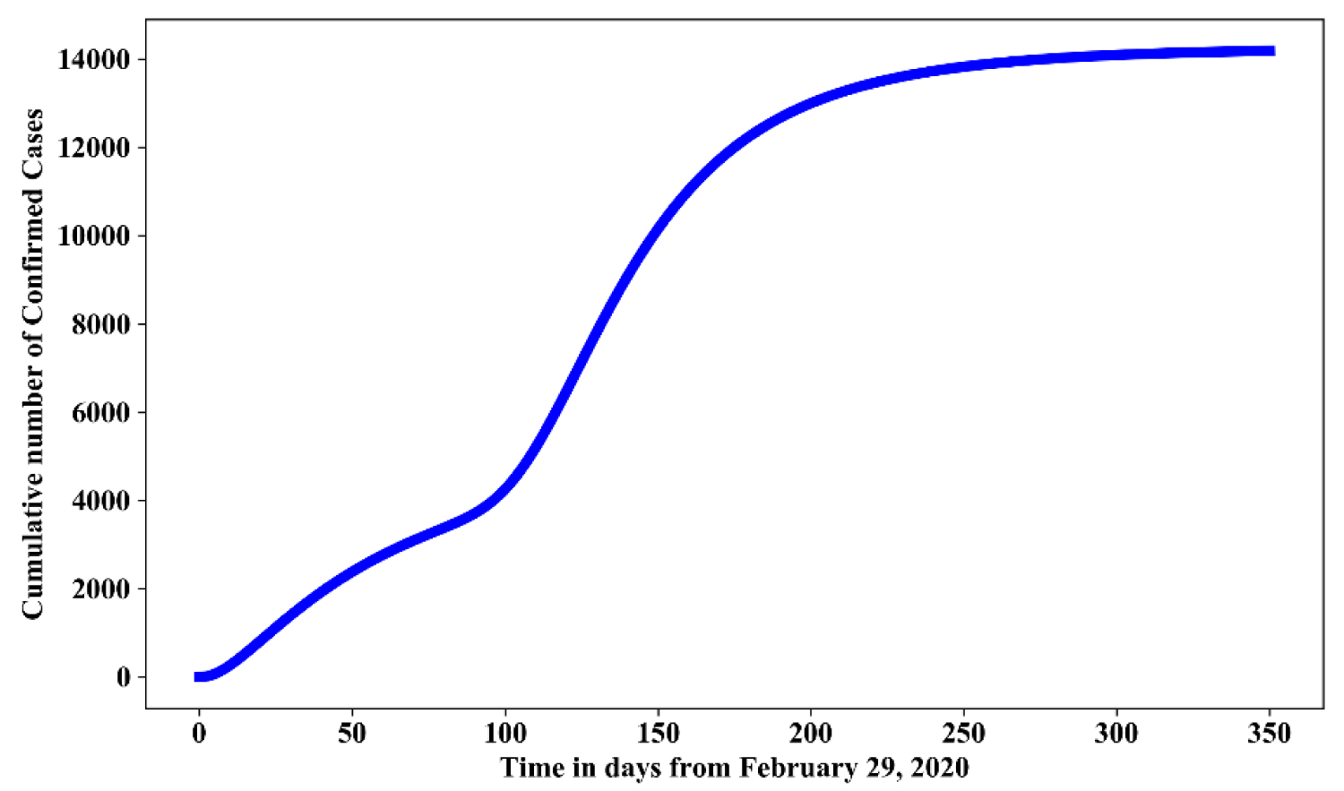 Figure 9: Simulation of model (1.1) for a full relaxation of lock down with 75% effective use of face mask and strict hygienic culture.
View Figure 9
Figure 9: Simulation of model (1.1) for a full relaxation of lock down with 75% effective use of face mask and strict hygienic culture.
View Figure 9
Hence, we suggest the following: wearing facial masks; maintaining social distance which could reduce the direct transmission; washing of hands to reduce indirect transmission; fumigation of the environment to reduce the virus from the environment; strict policy to combat the spread of the disease. This would be helpful to control the transmission of the virus.
The issue regarding reliability, precision and standard of the reported data are in short complex and out of the scope of this study, as this study is more focused on the aspect of mathematical modelling. Furthermore, since there is no data for the prevalence of the virus in the environment, we assumed 1/100000. This assumption might be overestimated or underestimated. Besides, the model is not age-structured and migration into and out of the country were not considered. Lastly, an individual infected with COVID-19 has the capability of transmitting the virus averagely to two other people in Nigeria, which implies an exponential rate between February 29, 2020 until when Nigeria government enforced lock down in populated States like Lagos State, Ogun State, Kano State, and the Federal Capital Territory, Abuja. In essence, before the lockdown is implemented (March 30, 2020 for Ogun State, Lagos State and FCT Abuja and May 12, 2020 for Kano State), many people has already been exposed, a large number of individuals in Nigeria may have died of COVID-19 during this period especially those with underlying conditions. Hence, there may be underreporting of confirmed cases and death reported especially during the period of lock down due to poor health system in Nigeria in terms of surveillance and level of testing. We plan to extend our model to study the spread of the COVID-19 in Nigeria in more details, predicting number of deaths and peak date predicted.
No funding was provided for this manuscript. Author declares no conflict of interest.