In order to overcome the difficulty in aligning specimens accurately within a reference system for angular kinematic measurements, a method of using a virtual reference coordinate system was designed and implemented in conjunction with using an optical motion capture device. The virtual coordinate system is created by digitizing three identifiable points in space. In this way, angular measurements of specimens can be described with respect to the virtual coordinate system to be anatomically relevant. This system provides an easier procedure for 3-D angular measurement than aligning the specimen with a loading apparatus, in which a reference coordinate system generally exists. More importantly, the procedure using a virtual reference coordinate system can diminish variations resulting from possible misalignments of specimens in a reference system, thus enabling reliable measurement of rotational data that is independent of specimen alignment.
The measurements of static and dynamic joint angular kinematics are used for a widespread range of applications, including biomechanical studies, sports performance, and rehabilitation [1]. The joint angular change refers to a rotational motion of the joints about the anatomical joint axes approximated by bony structures. Various methods, such as using goniometers, camera-based motion capturing systems, optical fibers, inertial sensors or radiographs, can be used for joint angle measurement [2-4]. These sensors or devices generally require the reference frames and test subjects or specimens that are aligned within the frames. The frames function as a reference coordinate system by which angular motion can be expressed. However, the accurate representation of angular change tends to be heavily contingent upon the alignment accuracy of the test subjects or specimens with respect to the reference frames. For example, in the application of ankle kinematics, small offsets in the alignment of an anatomical axis likely induce large errors of angular measurements describing joint rotations [5].
In order to improve the reliability of angular representation, as well as mitigate the difficulty of alignment procedures, a method of using a virtual reference coordinate system has been designed to be used in conjunction with a camera-based motion capturing system. Our proposed method allows for the joint angular measurements, with respect to the defined virtual reference coordinate system, has easily defined orientations of the virtual reference coordinate system in experimental setups. In addition, this provides more reliable measurement of rotational changes independent of alignment procedure with much less effort. This technical report focuses on the mathematical description for the proposed virtual reference coordinate system method and the validation of the method.
The method proposed in this report was developed to measure three-degrees of freedom joint angles (the rotation of x, y, and z axis, so called, yaw, pitch, and roll, respectively). This was designed and validated with the Optotrak system (Northern Digital Inc., Canada), but can work with other camera-based motion capturing systems. The Optotrak is a non-contact motion measurement system that tracks small infrared, light-emitting diodes that are attached to the test subjects.
Virtual points refer to points in space where it is difficult or undesirable to fix markers that are tracked by motion capturing systems. The virtual points can be individually defined by identifying specific points with a customized or commercial digitizing probe (Figure 1A). If three virtual points are specified in space, a virtual coordinate system can be created in such a manner that the x-axis is the line passing through the first and second virtual points, the y-axis is the line passing through the third virtual point and perpendicular to the x-axis (Figure 1B). For example, in ankle kinematics, a virtual coordinate system can be set up as follows: The first virtual point is defined at the tip of the lateral malleolus, the second point is at the tip of the medial malleolus, and the third point is relative to the anterior tibia above the foot. In this way, one of the axes will be aligned with the ankle anatomical axis because dorsi- and plantar-flexion of the foot are generally considered to take place in the ankle (talocrural) joint whose axis crosses the tips of lateral and medial malleolus [6-8].
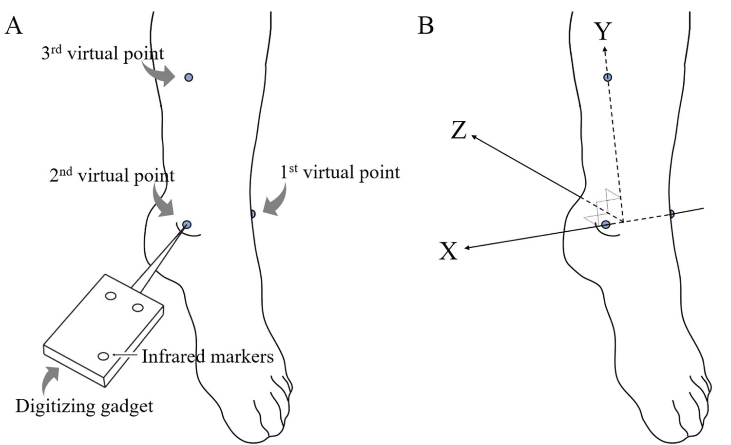 Figure 1: Virtual Coordinate System: A) Virtual points are defined in space by positioning a customized digitizing device to the tips of malleoli and a certain point in the tibia; B) The virtual coordinate system is set up in the way that the x-axis penetrated through the tips of malleoli, the y-axis is parallel to the lower limb, and the z-axis is created normal to the x- and y-axes.
View Figure 1
Figure 1: Virtual Coordinate System: A) Virtual points are defined in space by positioning a customized digitizing device to the tips of malleoli and a certain point in the tibia; B) The virtual coordinate system is set up in the way that the x-axis penetrated through the tips of malleoli, the y-axis is parallel to the lower limb, and the z-axis is created normal to the x- and y-axes.
View Figure 1
The accurate measurement of angular displacements of an object requires two coordinate systems: A referenced global coordinate system to describe the orientation of the object and a local coordinate system that is usually attached to the object being examined. For example, Figure 2A shows a pair of coordinate systems G and A, where the position and orientation of system A relative to G is defined by the displacement vector GA, and three unit vectors (GxA, GyA, and GzA) which align to the coordinate axes of the A coordinate system. For convenience, the three vectors are combined into a 3 × 3 matrix and written as GRA = [GxA GyA GzA], called a rotation matrix. The notation Ij is used to indicate the coordinates of a point j as expressed in a coordinate system I.
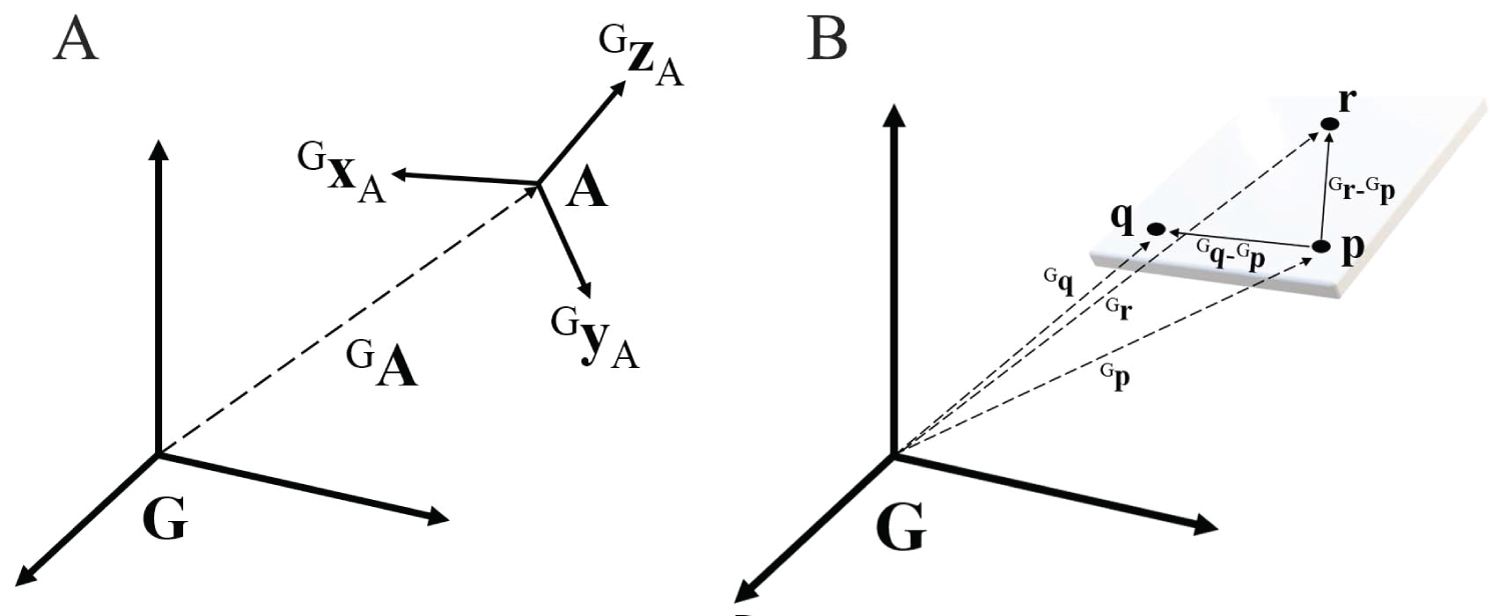 Figure 2: A) A pair of coordinate systems: the orientation of system A relative to G are defined by the three unit vectors (GxA, GyA, and GzA), combined and written as a 3 × 3 rotation matrix, GRA = [GxA GyA GzA], which completely describes the orientation of the A coordinate system with reference to the G coordinate system; B) Three points fixed on a rigid plane can set up an arbitrary local coordinate system, where one axis of the system is collinear to a vector pointing to a point from another point, and another axis is perpendicular to the plane.
View Figure 2
Figure 2: A) A pair of coordinate systems: the orientation of system A relative to G are defined by the three unit vectors (GxA, GyA, and GzA), combined and written as a 3 × 3 rotation matrix, GRA = [GxA GyA GzA], which completely describes the orientation of the A coordinate system with reference to the G coordinate system; B) Three points fixed on a rigid plane can set up an arbitrary local coordinate system, where one axis of the system is collinear to a vector pointing to a point from another point, and another axis is perpendicular to the plane.
View Figure 2
A rigid body can be made and attached to the object of interest to define a local coordinate system assigned to that object. The three-markers rigid bodies define three points in space which can be used to create a plan or set up a three-dimensional coordinate system. Since a rigid body contains three markers, it can constitute a plane in space, and an orthogonal coordinate system can be fixed to that plane. Figure 2B shows an example of a local coordinate system set up on a rigid plane containing three marker positions. With the position p as the origin of the local frame, the x-axis of the frame (i) can be defined as the same direction of the vector pointing to the point q from the point p (Gq-Gp). The y-axis of the frame (j) can be defined as perpendicular to the plane created by the three marker positions. The z-axis of the frame will then be automatically determined by the cross product i × j. The unit vectors (i, j, and k) along with the x, y, and z-axis of the local frame can be computed by the following formula:
This described procedure also applies to the process of obtaining virtual points using a digitizing probe. Since the three markers attached to the digitizing probe define a local coordinate system, and the physical location of the tip relative to the probe markers is already known, the tip position of the probe is easily measured.
In the application of ankle kinematics, two rigid bodies can be attached to the lower limb and the foot respectively, to define local coordinate systems assigned to each segment of the limb (Figure 3). The default global coordinate system (G) for the Optotrak system lies in the camera lens of the device, but any such camera-based capturing system has its own method for defining the global coordinate system. Any other coordinate systems that are specified on rigid bodies are therefore called local coordinate systems and are expressed with respect to the reference coordinate system. Figure 3 shows these coordinate systems defined for the application. We have defined four different coordinate systems for the kinematic measurement of ankle joint. The two local coordinate systems and the global coordinate system are denoted by A, B, and G respectively, and the virtual coordinate system is denoted by V. One of the axes of the virtual coordinate system is aligned with the anatomical joint axis. In this application, we aim to measure the foot angular motion (ankle rotation) about the anatomical axis, which is now replaceable by the V coordinate system.
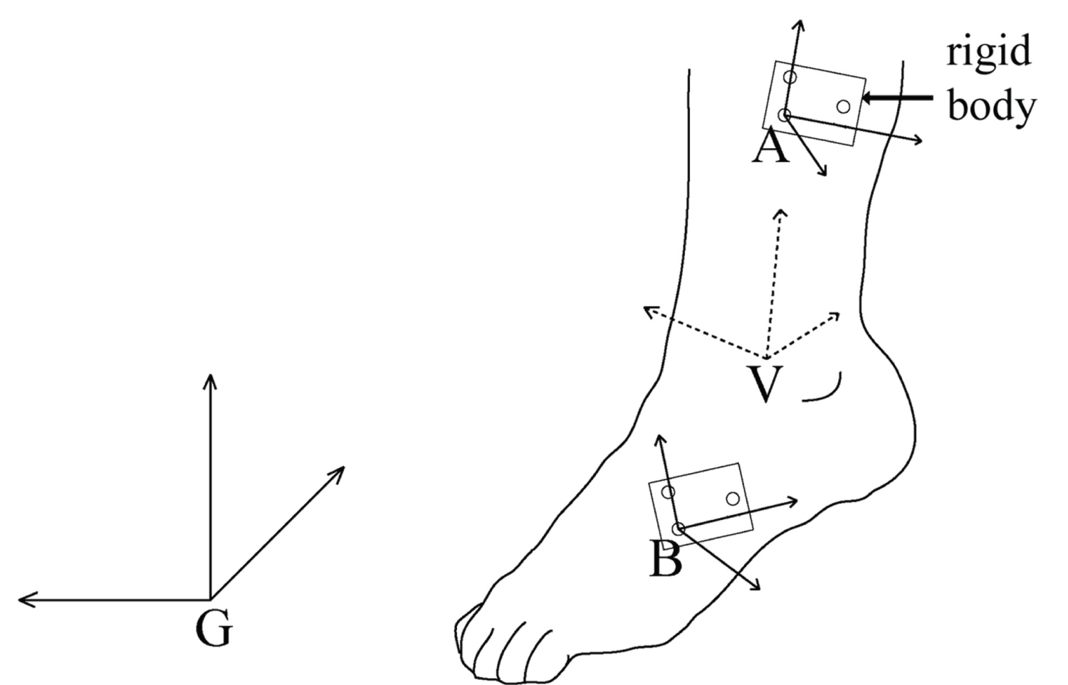 Figure 3: Coordinate systems defined for the kinematic measurement of ankle joint. G: The default global coordinates system, V: The defined virtual coordinate system. A and B: Two local coordinate systems set up using rigid bodies that contain three motion capture markers.
View Figure 3
Figure 3: Coordinate systems defined for the kinematic measurement of ankle joint. G: The default global coordinates system, V: The defined virtual coordinate system. A and B: Two local coordinate systems set up using rigid bodies that contain three motion capture markers.
View Figure 3
In order to make the measurement of the ankle rotation independent of any unintentional movement of the lower limb, the V coordinate system needs to be expressed with respect to the A coordinate system, that is fixed to the limb segment above the foot. Thus, the orientation of the V coordinate system needs to be represented by the rotation matrix ARV. The procedure in ARV computation is in the following description. Figure 4A shows the G, A, and V coordinate systems and the points P, Q, and R, the three virtual points that have been digitized previously. Based on these three points, the following vectors are defined: GP is a vector that begins at the origin of the G coordinate system and ends at point P, and similarly for GQ and GR. The notation Ij is used to indicate the coordinates of a point j as measured in a coordinate system I. By a principle of vector summation within the triangle, the virtual points P, Q, and R are now expressed in the A coordinate system as follows; AP = GP – GA, AQ = GQ – GA, and AR = GR – GA. As shown in Figure 4B, we can then create the x-axis of the V coordinate system along the line crossing the P and Q points, and the y-axis along the line crossing both R and the origin O, which is not defined yet.
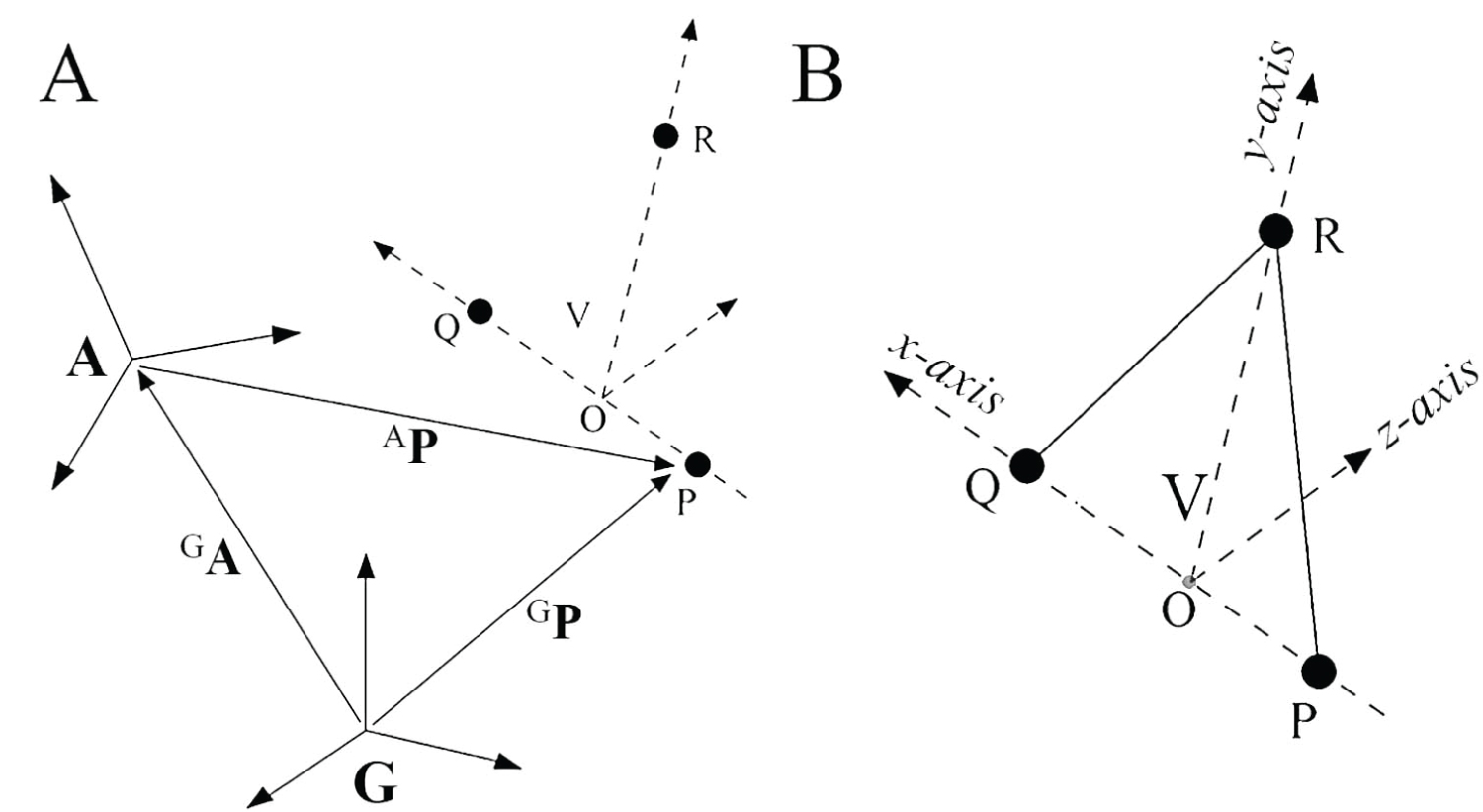 Figure 4: A) Illustration of the G, A, and V coordinate systems, and three virtual points P, Q, and R. The notation Ij is used to indicate the coordinates of a point j as measured in a coordinate system I. By a principle of vector summation within the triangle, the virtual points of P, Q, and R are expressed in the A coordinate system; B) Virtual coordinate system whose axes cross three points. The line crossing the P and Q points is the x-axis of the virtual coordinate system and the line crossing both R and the origin O is the y-axis.
View Figure 4
Figure 4: A) Illustration of the G, A, and V coordinate systems, and three virtual points P, Q, and R. The notation Ij is used to indicate the coordinates of a point j as measured in a coordinate system I. By a principle of vector summation within the triangle, the virtual points of P, Q, and R are expressed in the A coordinate system; B) Virtual coordinate system whose axes cross three points. The line crossing the P and Q points is the x-axis of the virtual coordinate system and the line crossing both R and the origin O is the y-axis.
View Figure 4
The origin O of the V coordinate system can be computed as follows. The O has coordinates and the vector from the origin of A to the origin O is written as AO = (AOx AOy AOz). Likewise, AP and AQ vectors are written as (APx APy APz) and (AQx AQy AQz), respectively. Since and is perpendicular (because x and y axes are orthogonal), the dot product of the two vectors gives ∙ . This is equivalent to the following scalar equation:
Also, the cross product of and will be perpendicular to (because z and y axis are orthogonal), so it gives . This is equivalent to the following scalar equation.
Lastly, since the virtual points P, O, and Q lie on the same line, the two vectors and are collinear . Thus, the ratios of distances of each component of the two vectors satisfies.
From the Equations (2), (3), and (4), the three coordinates (AOx, AOy, AOz) of the origin O can be obtained. Now that the vectors are known, the rotation matrix ARV can be written as
The orientations of the A and B local coordinate systems, with reference to the G coordinate system, are represented by GRA and GRB. Since motion capturing systems track the position of all markers in their default global coordinate system, the GRA and GRB are easily calculated from the marker information provided by the capturing system. The angular representation of the ankle between the foot and the limb segment above the foot must be independent of an unexpected movement of the limb segment during ankle motion. Therefore, an additional local coordinate system (A) has been assigned to the limb segment (above the foot) where the virtual coordinate system has also been set up. Now that the B coordinate system has been attached to the lower foot, VRB has the angular information about the anatomical ankle joint axis. The rotation matrix that relates the V and B coordinate systems is written as
Since VRA is an orthogonal matrix, it can be written as
On the other hand, GRB can be written as GRB = GRA ARB. When (GRA)-1 is taken on both sides, it yields (GRA )-1 GRB = (GRA)-1 GRA ARB. Since (GRA)-1 GRA = I, it finally gives
Substituting Equation (7) and (8) into the right side of the Equation (6), the VRB is finally calculated such as
Note that GRA and GRB are given from the measuring system, and the rotation matrix ARV can be easily obtained as described already. It is also important to note that the ARV is constant regardless of the motion of the limb segment above the foot if the A is still attached to the limb because the V and A coordinate systems have been already set up. In other words, the relative orientation of V with respect to A does not change even if the A coordinate system changes its position and orientation along the movement of the lower limb.
Figure 5A shows an example of the measurement of the ankle motion and shows the case of different orientation of the B coordinate system depending on the starting (B, when the foot is at a neutral position) and the next positions (B', after the foot is flexed). After foot movement, GRA' and GRB' can be computed using the new positions of markers in two rigid bodies. We now call the V coordinate system at the second measurement position V' (we assume that the limb segment above the foot moves slightly with the ankle movement). Using the Equation (9), the orientation of the B' coordinate system in the V' coordinate system can be computed as
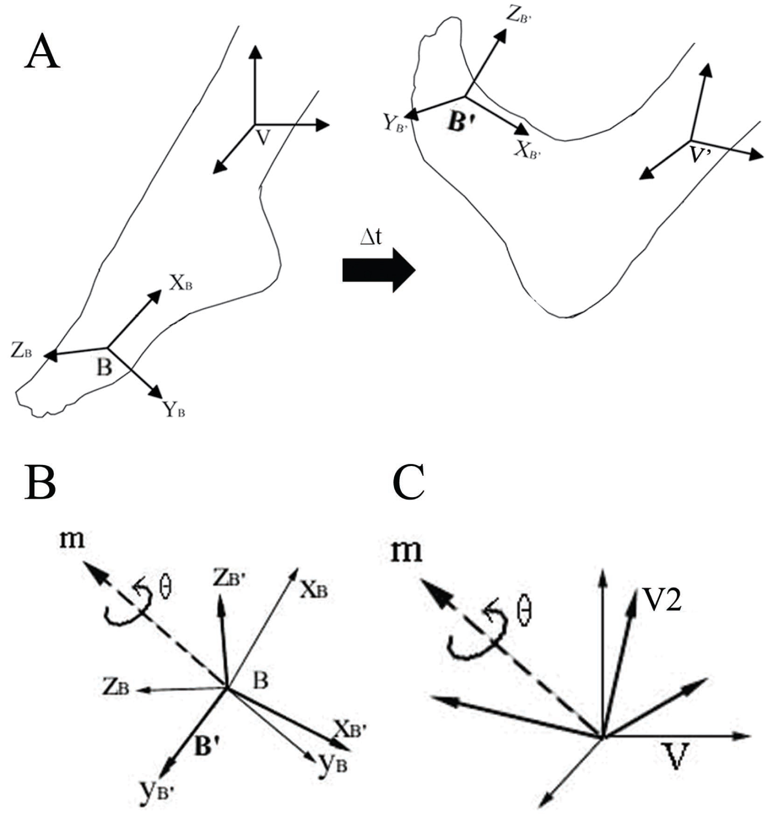 Figure 5: Change in Coordinate System with Ankle Position: A) This shows the change of the orientation of the B coordinate system, during a given interval time of Δt, between the starting position (B), when the foot hangs freely) and the next position (B', after the foot is flexed); B) The change of orientation of the B coordinate system can be regarded such that the B coordinate system is rotated about the vector of Bm by an angle of θ; C) The rotational axis Bm and angle θ are applied to the V coordinate system in a sense that the V coordinate system has been rotated to V2 during motion. Having calculated the rotation matrix VRV2 based on this, the successive rotations about the V coordinate system can be computed.
View Figure 5
Figure 5: Change in Coordinate System with Ankle Position: A) This shows the change of the orientation of the B coordinate system, during a given interval time of Δt, between the starting position (B), when the foot hangs freely) and the next position (B', after the foot is flexed); B) The change of orientation of the B coordinate system can be regarded such that the B coordinate system is rotated about the vector of Bm by an angle of θ; C) The rotational axis Bm and angle θ are applied to the V coordinate system in a sense that the V coordinate system has been rotated to V2 during motion. Having calculated the rotation matrix VRV2 based on this, the successive rotations about the V coordinate system can be computed.
View Figure 5
As already mentioned, the A'RV' will be the same as ARV. The computed VRB and V'RB' matrix describes the RPY angles (roll, pitch, and yaw), which represent successive rotations of the B and B' coordinate system about the fixed X, Y, and Z axes of the virtual reference coordinate system, respectively.
If the B local coordinate system would have been defined that their axes are exactly aligned to those of the V reference coordinate system at the starting position, the RPY angles computed from the V'RB' matrix would be the net angle components about the anatomical axis during the motion. However, this is not the usual case, and it is impractical to align the B with the V reference system whenever the measurements are made. Thus, in order to obtain the angular displacement of the joint at a given time with respect to a starting (neutral) position, we need to compute the orientation matrix described at both positions and calculate the net angle components occurring between the starting and the next position from those matrices.
The following procedure shows how to compute the net angle component. As shown in Figure 5B, the net change of the two matrices VRB and V'RB' can be represented by the unit vector Bm = [Bmx, Bmy, Bmz] and an angle of rotation θ. However, the final goal of this process is to express the net joint angles in the V reference coordinate system, instead of in the B coordinate system. Thus, the idea is that after determining the rotation axis Bm and angle θ in the B coordinate system, they can be applied to the V reference coordinate system such that V has been rotated during motion by an angle θ about the rotation axis Vm (Figure 5C).
Since BRB' = (GRB)-1 GRB', with the rotation matrix BRB', the rotation axis Bm and angle θ are obtained as follows [9]. If the rotation matrix BRB' is written as:
Solving for θ gives θ = cos-1((r00 + r11 + r22 -1)/2). The value of θ that lies in the range of 0 to π will be selected, and the unique corresponding axis of rotation will be computed (if the value of θ was in the range of -π to 0, the resulting rotation axis would point in the opposite direction to the one that will be computed).
Solving for Bm gives to (Bmx, Bmy, Bmz) as follows:
where, mx is positive if (r21-r12) is positive.
where, my is positive if (r02-r20) is positive.
where, mZ is positive if (r21-r12) is positive.
If the absolute value of mx is larger than the absolute values of my and mz, a more accurate answer for my and mz can be obtained by using a second term in the above formulas.
In order to express the measured rotation as a rotation that occurs within the V coordinate system, the rotation axis Bm and angle θ can be applied directly to the V coordinate system regardless of the orientation of the V coordinate system (Figure 5C). This allows the V coordinate system to be interpreted as rotating by θ around the axis of Bm. However, the Bm is the vector expressed in the B coordinate system. Thus, it needs to be expressed as a vector in the V coordinate system by Vm = VRB Bm. With Vm = (Vmx, Vmy, Vmz) and θ, the rotation matrix VRV' will be computed by using the following steps [9].
Where,
The roll, pitch, yaw (RPY) angles are successive rotations about the fixed XYZ axes, in that order:
Rzyx(γ, β, α) = Rz(γ)Ry(β)Rx(α)
Note that the order is right-to-left because of the rotation about the fixed axes. By contrast, Euler angles are successive rotations about the current axes. The results would be the same with the ZYX Euler angles. By comparing Equation (11) to Equation (12), the RPY angles of VRV' can be extracted as follows:
Finally, these three angles (between -90° and + 90°) are the net angular displacements of the lower foot from the first position B to the second position B' in the V reference coordinate system.
In order to demonstrate how the proposed method describes the useful information of joint angular changes in virtual reference system, we implemented the methods using a simple experimental instrument. Our proposed method in this study can be used for the measurement of any joint angles if its anatomical axis can be properly defined. Thus, we focused on validating our proposed method using a more generic and intuitive way than applying the method to actual joint measurements.
A camera-based motion capturing system (Optotrak) was used for method validation. Since the goal of this experiment was to focus on validating the method proposed in this study, the angular motion occurring in an experimental setup was measured rather than measuring the actual subject's joint motion (Figure 6). As shown in the figure, the first segment of the goniometer was fixed to a vertical wooden bar, and the lower segment of the goniometer can rotate. Two rigid bodies, A and B, were attached to the vertical bar and the rotating segment of the goniometer, respectively. The simple goniometer setup simulates a single-axis joint movement.
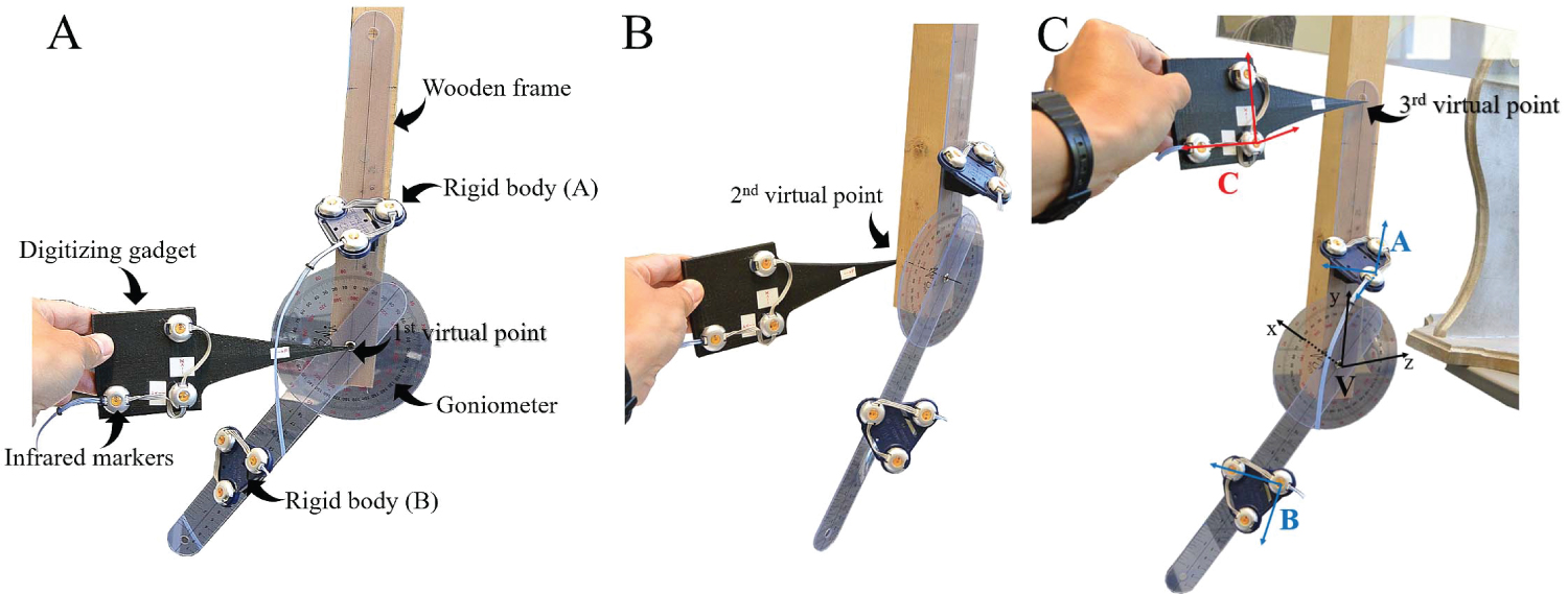 Figure 6: A) Experimental setup for method validation. A goniometer was fixed to a vertical wooden bar, and two rigid bodies were attached to the top and the lower frame of the goniometer. Each rigid body has three markers on it. The three virtual points were digitized as follows; the first one close to the center of the goniometer (A), the second one close to the other side of the goniometer rotating axis; B), and the third one somewhere on the top of the vertical bar; C) A total of four local coordinate systems including the one for the digitizing probe can be defined by the positions of actual markers and virtual markers as well.
View Figure 6
Figure 6: A) Experimental setup for method validation. A goniometer was fixed to a vertical wooden bar, and two rigid bodies were attached to the top and the lower frame of the goniometer. Each rigid body has three markers on it. The three virtual points were digitized as follows; the first one close to the center of the goniometer (A), the second one close to the other side of the goniometer rotating axis; B), and the third one somewhere on the top of the vertical bar; C) A total of four local coordinate systems including the one for the digitizing probe can be defined by the positions of actual markers and virtual markers as well.
View Figure 6
First, three virtual points were digitized. As shown Figure 6, the first virtual point was digitized as close as possible to the rotating center of the goniometer, the second virtual point was digitized close to the other side of the rotating axis (the opposite side of the wooden bar), and the last virtual point was digitized as the point about the middle of the top of the wooden bar. The tip of the 3D printed digitizing probe is 27.7 mm, 136.1 mm, and 7.9 mm away from the origin of the local digitizer coordinate system. By digitizing three virtual points in such a way, the rotating axis of the goniometer became closest to the x-axis of the virtual coordinate system, and the y-axis was defined in the upward direction of the vertical wooden bar (Figure 6C).
Next, for the measurement component of the experiment, 12 different angle changes were measured by moving the lower segment of the goniometer by 5° based on the neutral position (six angle changes were positive direction and the other six were negative direction). Figure 6A shows the neutral position (0°) of the goniometer. Thus, the total range of the angle changes was 60°. Only positions of markers fixed to rigid bodies A and B were recorded by the motion capturing system during these measurements: the process of digitizing virtual points was performed only once before different angle changes were measured.
Figure 7 shows the results of the validation test. All computation for the rotation matrices and angles were performed in MATLAB. The two local coordinate systems A and B were set up on the two rigid bodies (Figure 6C). Figure 7A shows the net rotation (θ) of the B co-ordinate system for each angle position about the neutral position of the goniometer. Mathematically, the net θ values were computed using BRB' (or VRV2). The calculated θ angles accurately corresponds to the angle changes read from the goniometer. The mean error across the 12 data points is 0.20° ± 0.12° and can be attributed to the reading error of the goniometer, not calculation error.
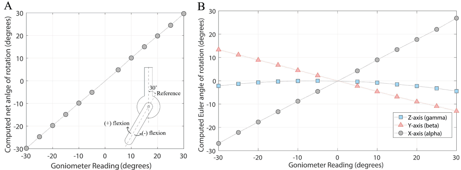 Figure 7: A) Computed rotation angle (about a single axis) for positive/negative rotations in the lower frame of goniometer. The x-axis of the graph shows the 12 different goniometer readings, and the y-axis shows the computed angles of rotation from the matrix BRB'; B) Computed ZYX Euler angles measured with respect to the virtual reference coordinate system for positive/negative rotations of the lower frame of goniometer.
View Figure 7
Figure 7: A) Computed rotation angle (about a single axis) for positive/negative rotations in the lower frame of goniometer. The x-axis of the graph shows the 12 different goniometer readings, and the y-axis shows the computed angles of rotation from the matrix BRB'; B) Computed ZYX Euler angles measured with respect to the virtual reference coordinate system for positive/negative rotations of the lower frame of goniometer.
View Figure 7
Figure 7B shows the computed ZYX Euler angles of the rotating segment in the virtual reference coordinate system (V). Since the x-axis of the virtual reference was close to the goniometer rotating axis, the X Euler angle (α) turned out to be most prominent. Note that the angle changes in Y-axis (β) and Z-axis (γ) indicate that the x-axis of the virtual reference system has not been completely parallel to the goniometer rotating axis. Overall, it was not our intention to make a perfect alignment between the goniometer rotating axis and one of the axes of the virtual reference system because the purpose of the experiment was to validate our proposed method.
A method that allows the measurement of three-dimensional joint angles without the need of careful sensor/specimen alignment was developed. In this method, a user can attach two rigid bodies (three markers each) with an arbitrary orientation. When defining a virtual reference coordinate system using three digitized points in space, the user can make one of the axes of the virtual reference coordinate system oriented align towards the joint anatomical axis. Then, the method algorithm computes the net angle changes by the specified axis. A camera-based capturing system was used to evaluate the performance of the proposed method, and the method proved to be robust and provided correct values.
In the cases where joint angular displacements are investigated about the anatomical or particular axes [10] having 3-D angular displacements described in a virtual reference coordinate system can provide many advantages. It will reduce the difficulty of careful alignment of a sensor or test specimen to a specific reference frame. Since small mistakes in the alignment have a strong impact on the measurement quality, our method can establish a more reliable and reproducible procedure for the measurement of joint angles. The virtual reference coordinate system can be easily created based on three digitally defined points in space. Net angle changes are then described with respect to the virtual reference coordinate system. Hence, this provides a convenient way to represent angular measurements in the user defined axes. Accordingly, it can diminish variations in angular measurements resulting from any possible misalignment of specimens in experimental setup. One limitation in the method application is that the anatomical axis of human joints made up a combination of bony structure, with which the virtual reference system is aligned, may slightly change without being fixed during motion. Although the joint axes may not be totally fixed during motion, clinically accepted joint axes are often considered stationary within a normal motion [6-8]. Another limitation is that rigid bodies should be held steady without being affected by any motions of subjects and the attachment of the rigid bodies should not affect the motions.
The proposed method has been applied to a biomechanical study where ankle kinematics were studied (not discussed here). The foot and lower foot were secured with 3D printed rigid bodies and LEDs in a pattern with known distances between them to establish local coordinate systems. In addition, a virtual anatomical coordinate system was calculated on the medial malleolus and tibia using the digitizer and rotation matrices. However, multiple joint kinematics can benefit from this method. A sound alignment procedure should be used for accurate joint kinematic data, and the alignment procedure using an anatomically relevant virtual coordinate system will provide more reliable and repeatable experimental results.
This work was supported by the Gordon and Jill Bourns College of Engineering at California Baptist University.
The authors declare that this study was conducted in the absence of any commercial or financial relationships that could be construed as a potential conflict of interest.