Artificial ankle joint replacement surgery is an important treatment for patients with ankle osteoarthritis (OA). Estimation of the pre-deformed ankle bones shapes are a key factor in artificial joint replacement surgery, and the surgeon can achieve highly satisfactory outcomes for patients such as less pain and sufficient function with an alternative ankle joint. However, the relationship between the bone shape deformation process and stage of the disease remains unclear. In this study, we investigated the relationship between the disease stage and three-dimensional rear foot bones (tibia, talus, and calcaneus) in patients with ankle OA.
Thirteen joints of eight women (69 ± 2 years) with OA and five healthy joints of five women (69 ± 2 years) with traumatic foot injury were investigated in this study. The images of the foot were captured using a Computed Tomography (CT) scanner, with the three-dimensional bone model created by stacking the CT images. In the control group, one left foot was randomly selected as the reference model. A three-dimensional cubic lattice deformation field was calculated from the three-dimensional bone model using the volume registration method to quantify the three-dimensional differences between the patients/subjects and the reference model. The relationship between the stage and shape was analyzed using principal component analysis (PCA).
In the tibia, the value of the first principal component corresponded to the curvature radius of the canopy surface shape, with a significant increase (p < 0.05) in the curvature radius of the tibia canopy surface in OA compared with the control group. In the talus, the value of the first principal component corresponded to the curvature radius of the subtalar joint surface, with a significant difference observed between the control and OA groups. The curvature radius of the subtalar joint surface tended to be larger in the OA group than in the control group.
Three-dimensional analysis using PCA revealed that the curvature radius of the tibia canopy surface increased in the OA group, similar to that observed in two-dimensional X-ray analysis. Furthermore, the proposed method revealed bones shapes deformation in the subtalar and ankle joints along three dimensions in the OA stage. Thus, the shape change of the tibia and talus could be evaluated three-dimensionally and quantitatively for each stage using the proposed method.
Volume registration, PCA, Tibia, Talus, Calcaneus, Ankle osteoarthritis
In recent years, Japan has become an aging society. According to a survey published in 2017 by the Cabinet Office, the population of elderly people aged 65 years and above was 35.15 million in 2016. The population of the elderly continues to increase, and it is estimated that this population will reach 38.78 million in 2042. Providing support for the independent living of elderly people is an important issue. Joint disease accounts for 11% of the total disease that necessitates the extension of support or primary nursing care to the elderly.
To continue independent living, it is important to care for the joints and treat joint disease properly [1-3]. Artificial joint replacement surgery [4-6] is one of the treatments for ankle osteoarthritis (OA) [6,7]. By replacing the artificial joint, the associated pain is removed/alleviated with recovery of ankle function. Artificial joint replacement surgery can be performed precisely by estimating the bone shape before progression of the ankle deformity. Using the estimated bone shape, an artificial ankle joint can be a highly satisfactory alternative with less pain and sufficient function. In a previous study, the alignment of the bones was evaluated from medical images obtained using a Computed Tomography (CT) [8,9], X-ray simple radiography apparatus (hereafter X-ray) [10,11], and magnetic resonance imaging (MRI) [12]. The data obtained from an X-ray is a two-dimensional fluoroscopic image, which depicts the image of the overlapping bone tissue projected from the object in the background. It is difficult to measure the three-dimensional data of the bone. Although MRI measurements can be acquired in three dimensions, it is difficult to extract the bones and analyze their three-dimensional structure using MRI. CT acquisitions can also be performed in three dimensions. It is difficult to analyze the three-dimensional structure from two-dimensional images.
In this study, the tibia, talus, and calcaneus of patients with ankle OA were analyzed three-dimensionally, and the relationship between the stage and shape was considered. Specifically, CT images were stacked to create a three-dimensional bone model. The volume registration method was used to quantify the deformation of the bone shape due to the progression of ankle OA as a displacement field. The relationship between the stage and shape was analyzed using principal component analysis (PCA) [13-15].
The data obtained using CT were primarily radiation transmission images. The image slices of the bones were in the Digital Imaging and Communication in Medicine (DICOM) format. In this experiment, the resolution and density resolution of the DICOM images were 512 × 512 pixels and 16 bits, respectively. The CT images of the right foot of each subject were reversed with respect to the sagittal plane. The right foot CT image group was made the same as the left foot image group. CT images of the left foot were acquired in all the subjects. In the healthy ankle group, one left foot was randomly selected as the reference model, while the others were marked as the target model. The three-dimensional bone model was created from the DICOM data. ITK-SNAP [16] was used to extract the 3D model in the stereolithography (STL) format by selecting and stacking the chosen area. A three-dimensional model of the bones were created for each subject, and the point cloud data of the bone was acquired.
The volume registration method was used to quantify the bone shape in each subject [17-19]. The volume registration method associates similar parts by calculating a deformation field that minimizes the luminance error of the two volumes. We employed the method that extends the registration method for 2D images proposed by Szeliski and Coughlan [14] to a 3D model. The calculated deformation field is expressed by a lattice three-dimensional space graphic. In this study, the deformation field was obtained by the expression method of the deformation field using spline interpolation. The deformation field of the entire volume can be described with a few variables, and the calculation cost can be reduced and stabilized. The deformation field necessary for deforming the reference model to a target model was calculated by using the volume registration method. This deformation field indicates deformation of the bone shape caused by the progression of OA. In this study, all three-dimensional volume data were preprocessed and three parameters, namely the origin, resolution, and sizes of the reference and target models were matched. The processing was performed according to the following procedure.
1. Using the anatomical feature points of the bone, the origin, X- and Y-axis directions were determined, and the Cartesian coordinate system was defined.
2. The image resolution of the volume was specified.
3. The volume was trimmed/truncated to 128 × 128 × 128 voxels.
4. Bone CT values were extracted and normalized to the range of 0 to 1.
Volume registration was performed on all three-dimensional volume data. Table 1 lists the parameters. The conditions for completing the iterative calculations were the same for all hierarchies. The calculation results of the bottom layer were considered as the final results. The calculations in the hierarchy ended when any of the following conditions was satisfied.
Table 1: Parameters when performing volume registration. View Table 1
• The least-square error e of the luminance value decreased three times consecutively to Dmin.
• The least square error e of the luminance value was less than Emin.
• The fudge factor of the Levenberg-Marquardt method was greater than λmax with the initial value set to 1.
• The number of iterations was greater than Imax,
The deformation field can be represented by a grid-like three-dimensional space figure. The deformation field is composed of control points. Each control point has an orthogonal displacement vector. As the evaluated image data had a volume of 128 × 128 × 128 voxels, the number of control points was 4913 (17 × 17 × 17), with 14739 degrees of freedom. The control point displacement quantifies the difference in shape between the two volumes.
Figure 1 shows the deformation field, where (A) and (B) show the states before and after deformation, respectively. This study aimed to evaluate the change in the shape of each bone. When the amount of displacement was calculated in a space portion other than the bone shape, the accuracy of the statistical analysis was affected. Therefore, as shown in Figure 2, the amount of displacement (other than the bone) was set to 0.
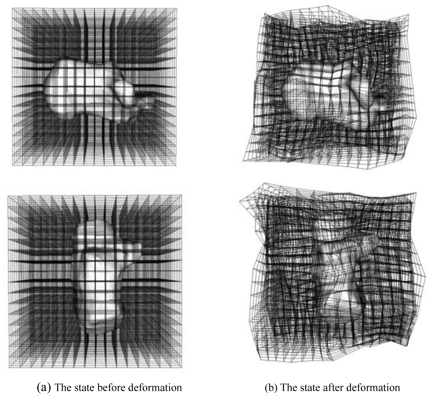 Figure 1: The state of the deformation field. The deformation field is represented by a grid-like three-dimensional space figure. The deformation field is composed of control points. Since the used image data has a volume size of 128 × 128 × 128 [voxel], the number of control points is 4913 (17 × 17 × 17), and the total degree of freedom is 14739.
View Figure 1
Figure 1: The state of the deformation field. The deformation field is represented by a grid-like three-dimensional space figure. The deformation field is composed of control points. Since the used image data has a volume size of 128 × 128 × 128 [voxel], the number of control points is 4913 (17 × 17 × 17), and the total degree of freedom is 14739.
View Figure 1
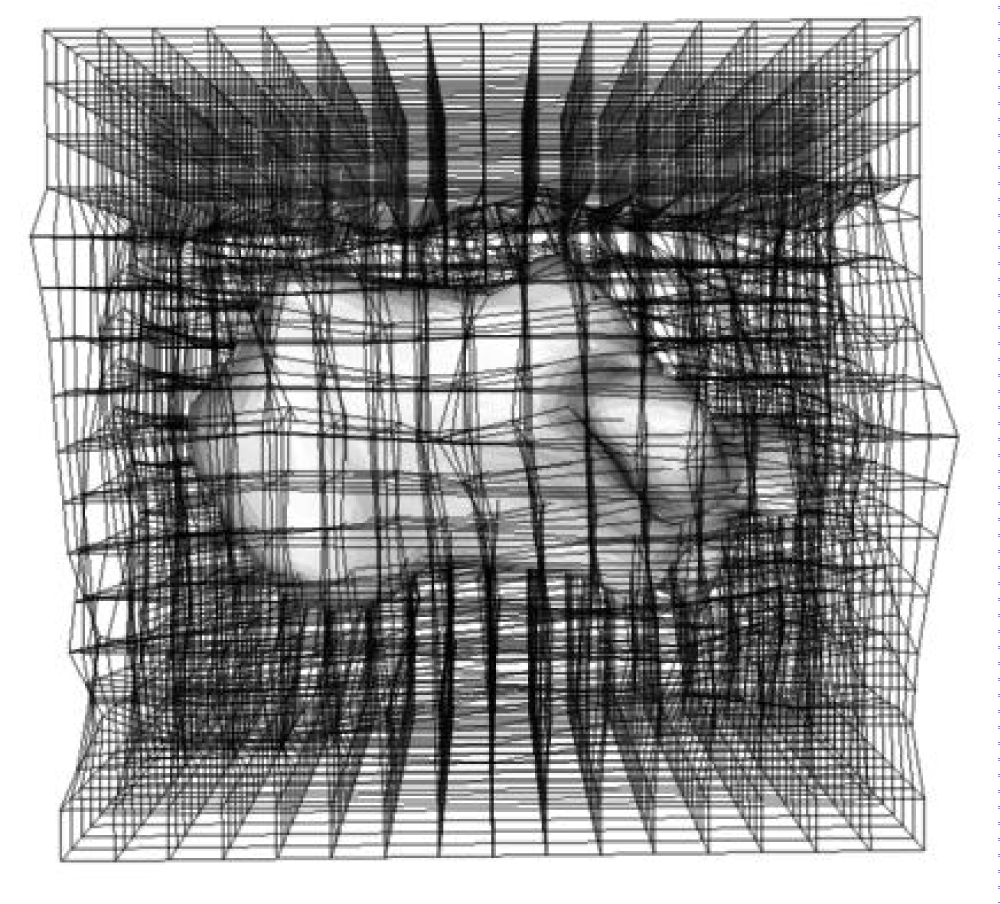 Figure 2: The state of the displacement amounts other than the bone is set to 0. Similar processing was performed on the bones to be analyzed (tibia, talus, and calcaneus).
View Figure 2
Figure 2: The state of the displacement amounts other than the bone is set to 0. Similar processing was performed on the bones to be analyzed (tibia, talus, and calcaneus).
View Figure 2
To investigate deformation of the bone shape due to the progression of arthropathy, PCA was performed on the displacement field.PCA was employed to reduce dimension, extract features, compress data, and identify key factors as the principal components. PCA converts variables with characteristic variations in the displacement fields to principal components. Each principal component visualizes the geometric variations of a subject. Each principal component can be visualized by changing the weights of each component. Based on the results of PCA, bones were created and the bone shape changed with OA. Specifically, it was assumed that the deformation field necessary to deform from the reference model to subject k can be calculated at n control points.
If the displacement of the first control point is (x1, y1, z1), then the displacement field at n control points can be calculated using Equation (1).
The total number of subjects is defined as p. The average shape vector m, which is the average of the deformation field vectors of all subjects, can be expressed by Equation (2).
Equation (3) defines a matrix D that can be calculated based on the deviation of the deformation vector and the mean vector, to transform the reference model into the target model.
The principal components representing the shape features can be computed by an eigenvalue decomposition of this variance-covariance matrix. The vector di', which represents the deformation field, is expressed in terms of the average vector m and calculated principal component, as defined in Equation (4). This enables visualization of the corresponding shape feature of the i-th principal component.
Where ci is the computed i-th eigenvector, and α is the weighting factor for the principal component.
Figure 3 shows the model generated from the displacement field obtained by the volume registration method. The model generated by the proposed method was calculated to be equivalent to the target analysis model. Therefore, the volumes of the generated and target analysis models should match. The reproduction accuracy was verified in ten subjects by comparing the volumes of the generated and target analysis models. The results are shown in Table 2. The average accuracy rate was 85%. By examining the results individually, it can be seen that the correct answer rate was 66.9% and 70.2%, which was lower than that of the other models. The two models were Stage 3B and Stage 4. The surface shapes of Stage 3B and Stage 4 were deformed owing to the deformation of the bone. In this study, we focused on a significant change, such as a change in the curvature of the bone, as opposed to a small change in the shape of the surface. Therefore, small surface deformations were ignored. After removing the two models, the accuracy rate was approximately 90%, which was considered sufficiently accurate.
Table 2: Accuracy of volume registration. The source model indicates the volume of the source model deformed using the result of the volume registration. The target model indicates the volume of the bone to be analyzed. View Table 2
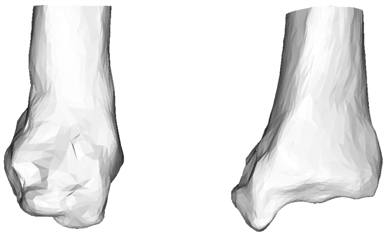 Figure 3: Generated tibia model using mean deformed grid. The model is generated by adding the deformation field calculated by volume registration to the source model.
View Figure 3
Figure 3: Generated tibia model using mean deformed grid. The model is generated by adding the deformation field calculated by volume registration to the source model.
View Figure 3
Ankle OA patients were classified into 5 stages using the Takakura and Tanaka classification [6]. In this study, Stage 1 with no joint space in the CT image was diagnosed as a healthy ankle joint. The number of joints in each stage was one joint in Stage 1, three joints in Stage 2, three joints in Stage 3A, five joints in Stage 3B, and two joints in Stage 4. The average age was 69 (± 2 years) for the healthy subjects and 69 (± 2 years) for patients with ankle OA.
In this study, images of the foot were captured/acquired using a CT scanner (Optimal CT 600, GE Healthcare Inc.). While capturing the CT and MRI images of patients with disease in the ischium and intervertebral disc, a medical compressor was used for the diagnosis of lumbar vertebra. In this study, a medical compressor was used to maintain a resting stance position when the subjects were in the supine position during CT acquisition. There was no significant difference in the center of plantar pressure between this condition and standing [20]. The photographed interval was 0.625 [mm]. By inverting the right foot images of each subject with respect to the sagittal plane, these images were assigned to the left foot images in the captured image group. This ensured that the CT image group of the right foot was equivalent to the image group of the left foot. The CT images were acquired at Heisei Memorial Hospital, which is a social medical corporation under the cooperation of Nara Prefectural University of Medical University.
Figure 4 shows the contribution rate and cumulative contribution rate in the PCA of the shape of the tibia. The cumulative contribution rate was greater than 80% up to the seventh principal component. In general, the principal component was adopted so that the cumulative contribution rate exceeded 80%, and the results were interpreted. Therefore, the study uses up to the 7th principal component. To visualize the features represented by each principal component, the three-dimensional target model can be deformed in the deformation field with the displacement vector calculated in Equation. (4).
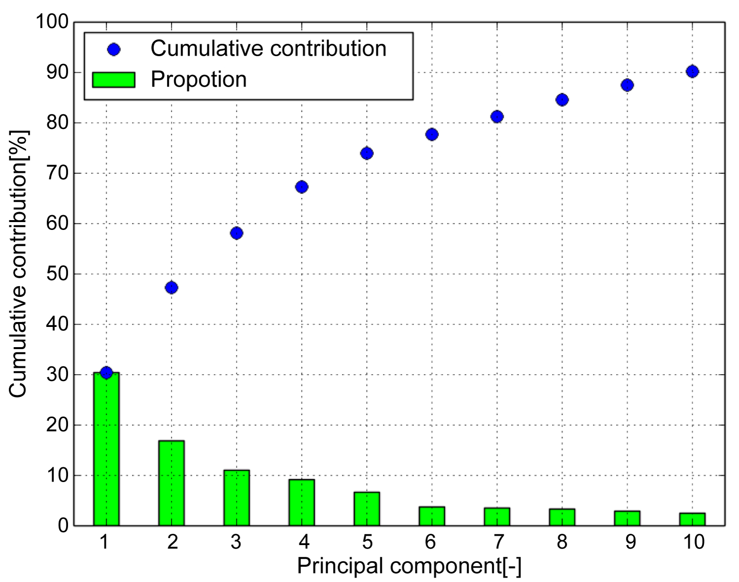 Figure 4: Cumulative contribution (Tibia). Cumulative contribution rate exceeded 80 [%] up to the seventh principal component. Therefore, use up to the 7th principal component.
View Figure 4
Figure 4: Cumulative contribution (Tibia). Cumulative contribution rate exceeded 80 [%] up to the seventh principal component. Therefore, use up to the 7th principal component.
View Figure 4
The weighting factor was set to +2σi or −2σi to highlight the differences in the features. σi is the standard deviation of the i-th principal component score. Consequently, some features, as shown in Figure 5, were identified, where (A) Is the first principal component corresponding to the canopy surface, (B) Is the second principal component corresponding to the curvature of the coronal plane, (C) Is the third principal component corresponding to the curvature of the sagittal plane, (D) Is the fourth principal component corresponding to the articular surface of the medial malleolus, and (E) Is the fifth principal component corresponding to the thickness of the tibia. However, these remarkable results include various shape features. In addition, as the shape characteristics of the sixth and seventh principal components cannot be described briefly, this will not be included in this article.
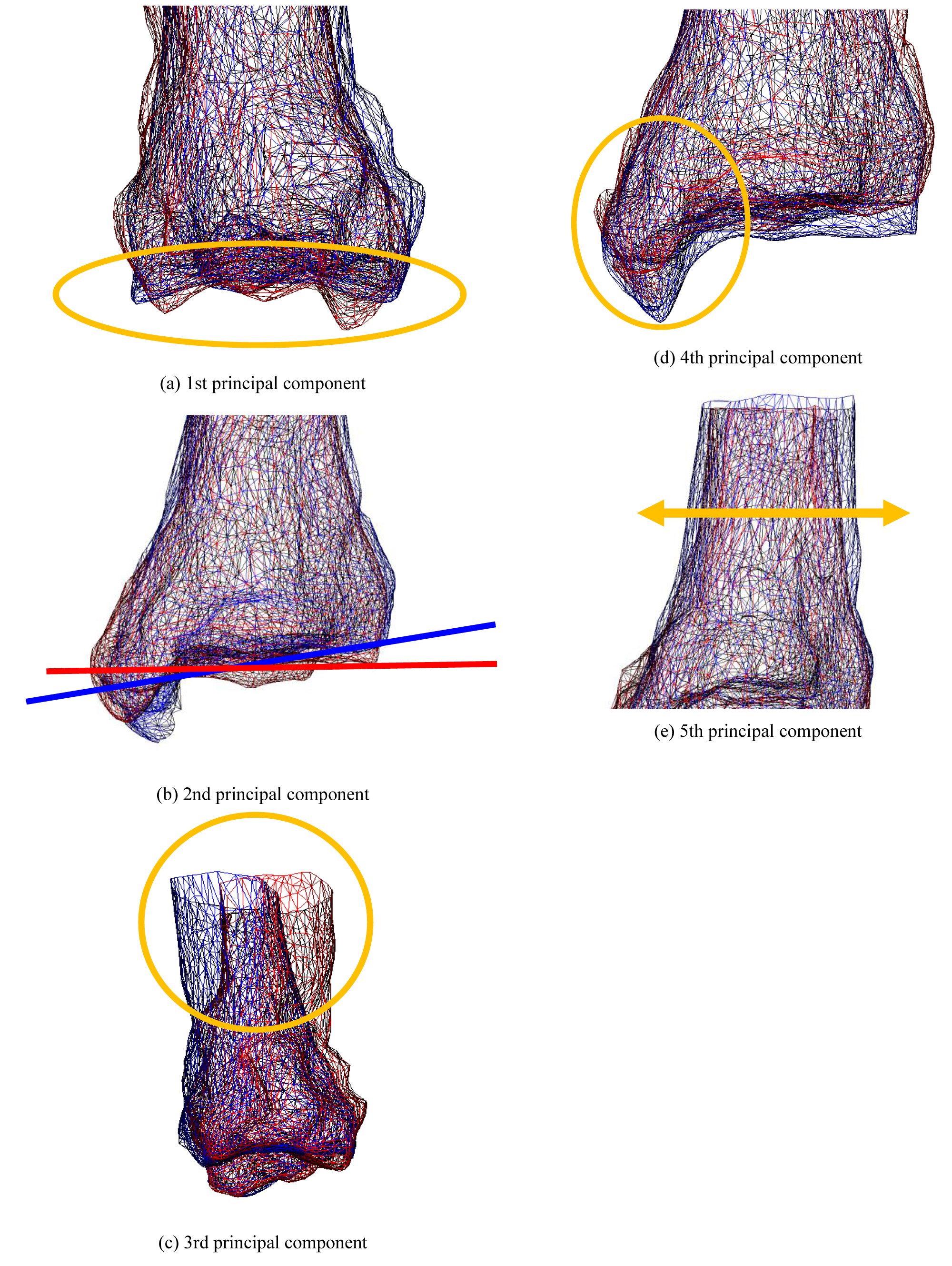 Figure 5: The state of deformation of the target model (Tibia). Each bone shows a bone when the weight of the principal component is ± 2σ. Red bones indicate + 2σ, and blue bones indicate -2σ.
View Figure 5
Figure 5: The state of deformation of the target model (Tibia). Each bone shows a bone when the weight of the principal component is ± 2σ. Red bones indicate + 2σ, and blue bones indicate -2σ.
View Figure 5
Figure 6 shows the shape distribution with the first principal component on the horizontal axis and the second principal component on the vertical axis. The central corner marker represents the average shape of all subjects. The blue corner marker in the graph represents the average shape of the tibia of a healthy ankle joint. The ellipse in Figure 6 is the 2σ probability ellipse, which statistically corresponds to a range of 95.4%. The yellow-green ellipse represents 95.4% of the tibia of all subjects, while the blue ellipse corresponds to 95.4% when considering the tibia of a healthy ankle joint. It can be observed that the opening of the canopy surface narrowed as the score of the first principal component increased. The healthy group was found to be distributed in the positive part of the first principal component, while the OA group was distributed in the negative part. It can be seen that the curvature of the coronal plane increased as the score of the second principal component decreased. A uniform distribution was obtained regardless of whether the ankle joint was a healthy or OA ankle.
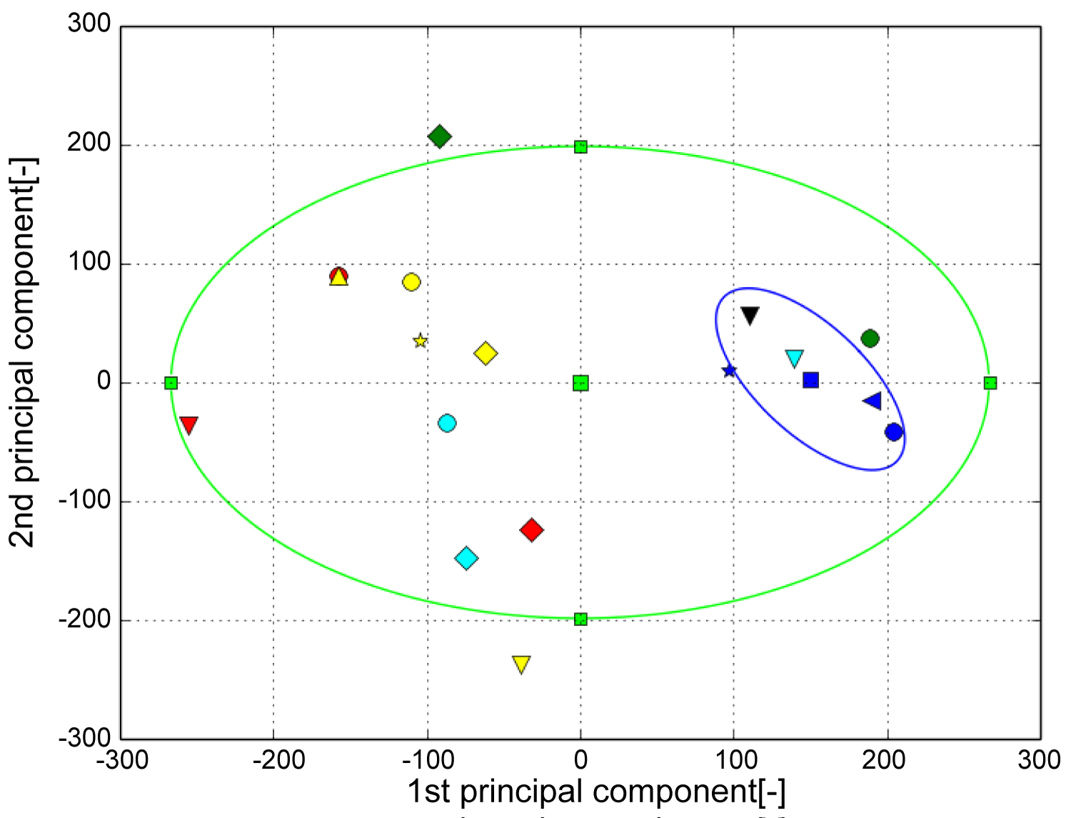 Figure 6: The result of PCA (Tibia). The horizontal axis represents the first principal component and the vertical axis represents the second principal component. The green ellipse is the probability ellipse and indicates the area that occupies 95% of all subjects, and the blue ellipse indicates the area that occupies 95% of healthy subjects. Blue is healthy, Black is Stage 1, Green is Stage 2, Light blue is Stage 3A, Yellow is Stage 3B, Red is Stage 4.
View Figure 6
Figure 6: The result of PCA (Tibia). The horizontal axis represents the first principal component and the vertical axis represents the second principal component. The green ellipse is the probability ellipse and indicates the area that occupies 95% of all subjects, and the blue ellipse indicates the area that occupies 95% of healthy subjects. Blue is healthy, Black is Stage 1, Green is Stage 2, Light blue is Stage 3A, Yellow is Stage 3B, Red is Stage 4.
View Figure 6
Figure 7 shows the contribution rate and cumulative contribution rate in the PCA of the talus shape. The cumulative contribution rate was greater than 80% up to the seventh principal component. Figure 8 shows the state of deformation of the target model, where (A) Is the first principal component corresponding to the shape of the subtalar joint, (B) Is the second principal component corresponding to the flattening of the pulley surface, (C) Is the third principal component corresponding to the size of the talus, (D) Is the fourth principal component corresponding to lateral protrusion and neck swelling, and (E) Is the seventh principal component corresponding to the medial subtalar joint surface. As the shape characteristics of the fifth and sixth principal components cannot be described briefly, these characteristics will not be discussed in this article.
 Figure 7: Cumulative contribution (Talus). Cumulative contribution rate exceeded 80 [%] up to the seventh principal component. Therefore, use up to the 7th principal component.
View Figure 7
Figure 7: Cumulative contribution (Talus). Cumulative contribution rate exceeded 80 [%] up to the seventh principal component. Therefore, use up to the 7th principal component.
View Figure 7
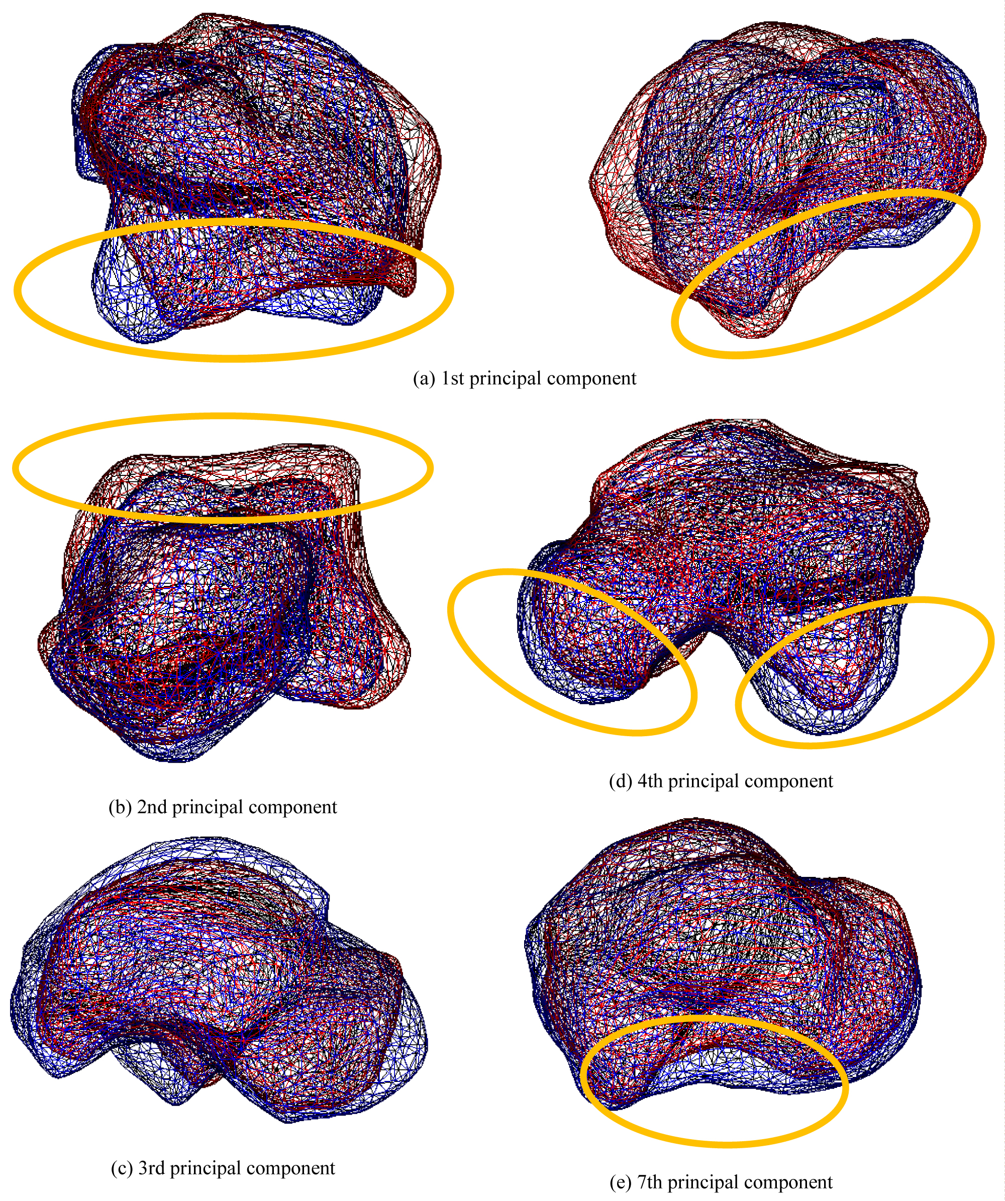 Figure 8: The state of deformation of the target model (Talus). Each bone shows a bone when the weight of the principal component is ± 2σ. Red bones indicate + 2σ, and blue bones indicate -2σ.
View Figure 8
Figure 8: The state of deformation of the target model (Talus). Each bone shows a bone when the weight of the principal component is ± 2σ. Red bones indicate + 2σ, and blue bones indicate -2σ.
View Figure 8
Figure 9 shows the shape distribution with the first principal component on the horizontal axis and second principal component on the vertical axis. It can be observed that the subtalar joint surface flattened as the score of the first principal component increased. The OA group was distributed in the positive part of the first principal component, while the healthy group was distributed in the negative part. It can be seen that the talus pulley flattened as the score of the second principal component decreased. The healthy group was distributed in the positive part of the first principal component, while the OA group was distributed in the negative part.
 Figure 9: The result of PCA (Talus). The horizontal axis represents the first principal component and the vertical axis represents the second principal component. The green ellipse is the probability ellipse and indicates the area that occupies 95% of all subjects, and the blue ellipse indicates the area that occupies 95% of healthy subjects. Blue is healthy, Black is Stage 1, Green is Stage 2, Light blue is Stage 3A, Yellow is Stage 3B, Red is Stage 4.
View Figure 9
Figure 9: The result of PCA (Talus). The horizontal axis represents the first principal component and the vertical axis represents the second principal component. The green ellipse is the probability ellipse and indicates the area that occupies 95% of all subjects, and the blue ellipse indicates the area that occupies 95% of healthy subjects. Blue is healthy, Black is Stage 1, Green is Stage 2, Light blue is Stage 3A, Yellow is Stage 3B, Red is Stage 4.
View Figure 9
Figure 10 shows the contribution rate and cumulative contribution rate in the PCA of the calcaneus shape. The cumulative contribution rate exceeded 80% up to the eighth principal component.
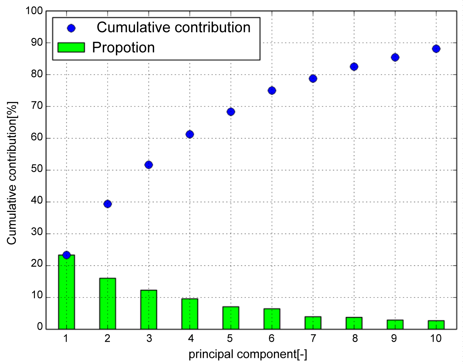 Figure 10: Cumulative contribution (Calcaneus). Cumulative contribution rate exceeded 80 [%] up to the seventh principal component. Therefore, use up to the 8th principal component.
View Figure 10
Figure 10: Cumulative contribution (Calcaneus). Cumulative contribution rate exceeded 80 [%] up to the seventh principal component. Therefore, use up to the 8th principal component.
View Figure 10
Figure 11 shows the deformation state of the target model, where (A) Is the first principal component corresponding to swelling of the proximal portion relative to the articular surface of the cuboid, (B) Is the second principal component corresponding to the shape of the subtalar joint, (C) Is the third principal component corresponding to swelling of the proximal part from the posterior talar articular surface, (D) Is the fourth principal component corresponding to the expansion of the calcaneus bulge, and (E) Is the seventh principal component corresponding to the length in the sagittal plane. As the shape characteristics of the fifth, sixth, and eighth principal components cannot be described briefly, this will not be included in this article.
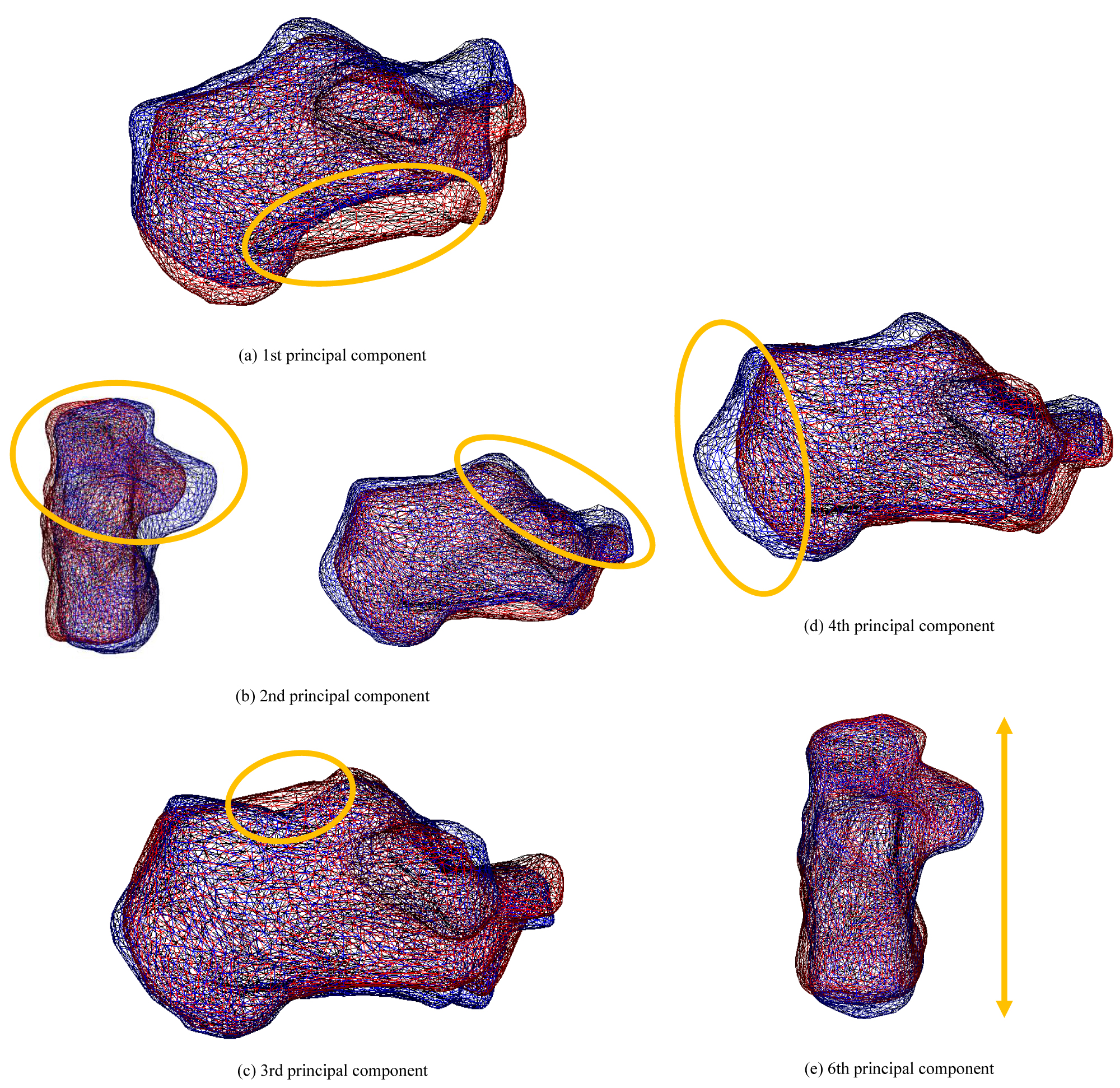 Figure 11: The state of deformation of the target model (Calcaneus). Each bone shows a bone when the weight of the principal component is ± 2σ. Red bones indicate + 2σ, and blue bones indicate -2σ.
View Figure 11
Figure 11: The state of deformation of the target model (Calcaneus). Each bone shows a bone when the weight of the principal component is ± 2σ. Red bones indicate + 2σ, and blue bones indicate -2σ.
View Figure 11
Figure 12 shows the shape distribution with the first principal component on the horizontal axis and second principal component on the vertical axis. It can be observed that the proximal part swelled relative to the cuboid joint surface as the score of the first principal component increased. It can be seen that the subtalar joint surface shrank as the score of the second principal component increased. A uniform distribution was obtained regardless of whether the ankle joint was a healthy or OA ankle.
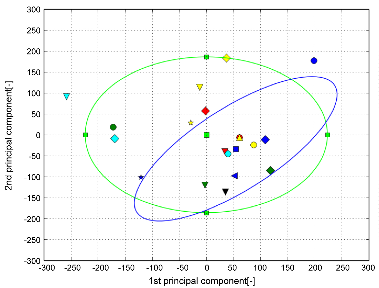 Figure 12: The result of PCA (Calcaneus). The horizontal axis represents the first principal component and the vertical axis represents the second principal component. The green ellipse is the probability ellipse and indicates the area that occupies 95% of all subjects, and the blue ellipse indicates the area that occupies 95% of healthy subjects. Blue is healthy, Black is Stage 1, Green is Stage 2, Light blue is Stage 3A, Yellow is Stage 3B, Red is Stage 4.
View Figure 12
Figure 12: The result of PCA (Calcaneus). The horizontal axis represents the first principal component and the vertical axis represents the second principal component. The green ellipse is the probability ellipse and indicates the area that occupies 95% of all subjects, and the blue ellipse indicates the area that occupies 95% of healthy subjects. Blue is healthy, Black is Stage 1, Green is Stage 2, Light blue is Stage 3A, Yellow is Stage 3B, Red is Stage 4.
View Figure 12
The bone shape characteristics of patients with OA were analyzed by statistical analysis of the quantified bones shapes. Statistical analysis of the tibia showed that it corresponded to the shape of the tibial canopy surface. The observation of the articular surface supported the report that the canopy surface is open forward and stress is concentrated in patients with arthropathy [8].
A low principal component score indicated opening of the canopy surface. In stages 3B and 4 with low scores, joint surface opening was confirmed. It was suggestive that the tibia deforms with disease progression. In addition, the statistical analysis of the talus showed that it corresponded to the shape of the subtalar joint. A high principal component score indicated joint flatness. This suggests that the subtalar joint is important for ankle stability. While previous studies have reported that the subtalar joint functions to compensate for the deformation of the talus joint caused by arthropathy, this study supports this mechanism from the perspective of the three-dimensional talus shape. Future studies should also include larger samples, as our results were likely impacted by the relatively small sample size and between-subjects variability. Despite these limitations, this study provides the first objective and quantitative description of three-dimensional bones shapes deformation in the subtalar and ankle joints in the OA stage.
In this study, the tibia, talus, and calcaneus of patients with ankle OA were three-dimensionally analyzed, and the relationship between the stage and shape was investigated. The volume registration method was used to quantify bone shape deformation and was statistically analyzed using PCA. In addition to the available two-dimensional images, results supporting disease mechanism based on the three-dimensional shape were obtained. Future studies will focus on evaluating larger datasets to obtain higher accuracy, facilitating its potential use in medicine.